Kaggle Earthquake Database
Here’s a map of earthquake location and magnitude (>=5.5) from 1965-2016. The data may be found on Kaggle.
Simple feature collection with 6 features and 19 fields
Geometry type: POINT
Dimension: XY
Bounding box: xmin: -173.972 ymin: -59.076 xmax: 166.629 ymax: 19.246
Geodetic CRS: +proj=longlat +datum=WGS84 +no_defs +ellps=WGS84 +towgs84=0,0,0
# A tibble: 6 × 20
Date Time Type Depth `Depth Error` Depth Seismic Statio…¹ Magnitude
<date> <time> <chr> <dbl> <dbl> <dbl> <dbl>
1 1965-02-01 13:44:18 Eart… 132. NA NA 6
2 1965-04-01 11:29:49 Eart… 80 NA NA 5.8
3 1965-05-01 18:05:58 Eart… 20 NA NA 6.2
4 1965-08-01 18:49:43 Eart… 15 NA NA 5.8
5 1965-09-01 13:32:50 Eart… 15 NA NA 5.8
6 1965-10-01 13:36:32 Eart… 35 NA NA 6.7
# ℹ abbreviated name: ¹`Depth Seismic Stations`
# ℹ 13 more variables: `Magnitude Type` <chr>, `Magnitude Error` <dbl>,
# `Magnitude Seismic Stations` <dbl>, `Azimuthal Gap` <dbl>,
# `Horizontal Distance` <dbl>, `Horizontal Error` <dbl>,
# `Root Mean Square` <dbl>, ID <chr>, Source <chr>, `Location Source` <chr>,
# `Magnitude Source` <chr>, Status <chr>, geometry <POINT [°]>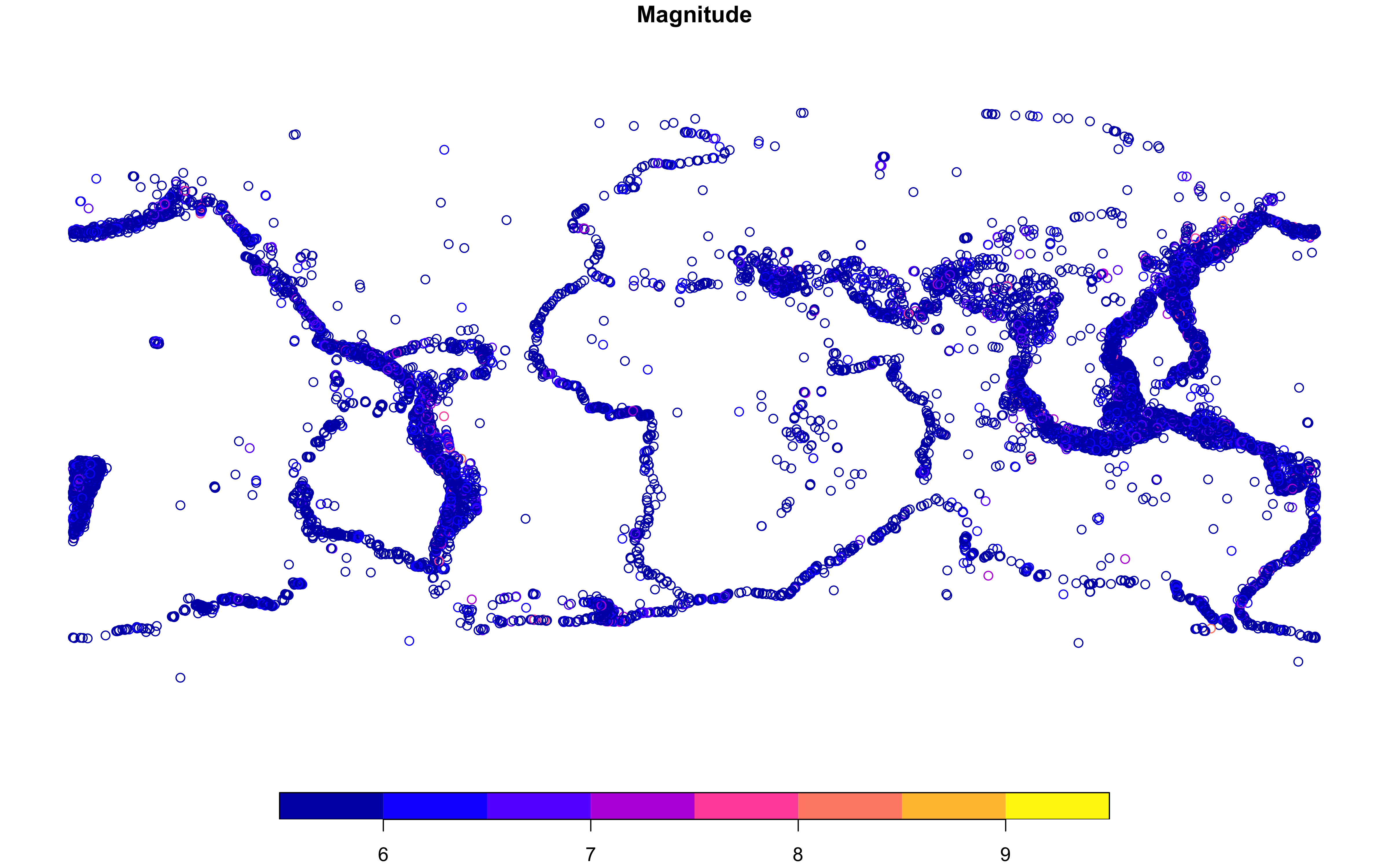
ggplot() +
  geom_sf(data = world_1, colour = "grey60", fill = "grey70") +
  geom_sf(data = quakes_sf_trans, aes(colour = Magnitude, size = Magnitude),
    stat = "sf_coordinates",
    shape = "*", alpha = 0.4) +
  scale_colour_viridis_c(option = "mako", direction = 1) +
  guides(size = "none",
    colour = guide_colourbar(title = "Magnitude",
      title.position = "left")) +
  coord_sf(expand = FALSE) +
  labs(x = NULL, y = NULL,
    title = "The Kaggle Earthquake Data",
    subtitle = "Significant Earthquakes, 1965-2016") +
  theme_minimal() +
  theme(
    panel.grid.major = element_line(colour = "grey90"),
    legend.background = element_blank(),
    legend.title = element_text(angle = 90),
    legend.title.align = 0.5)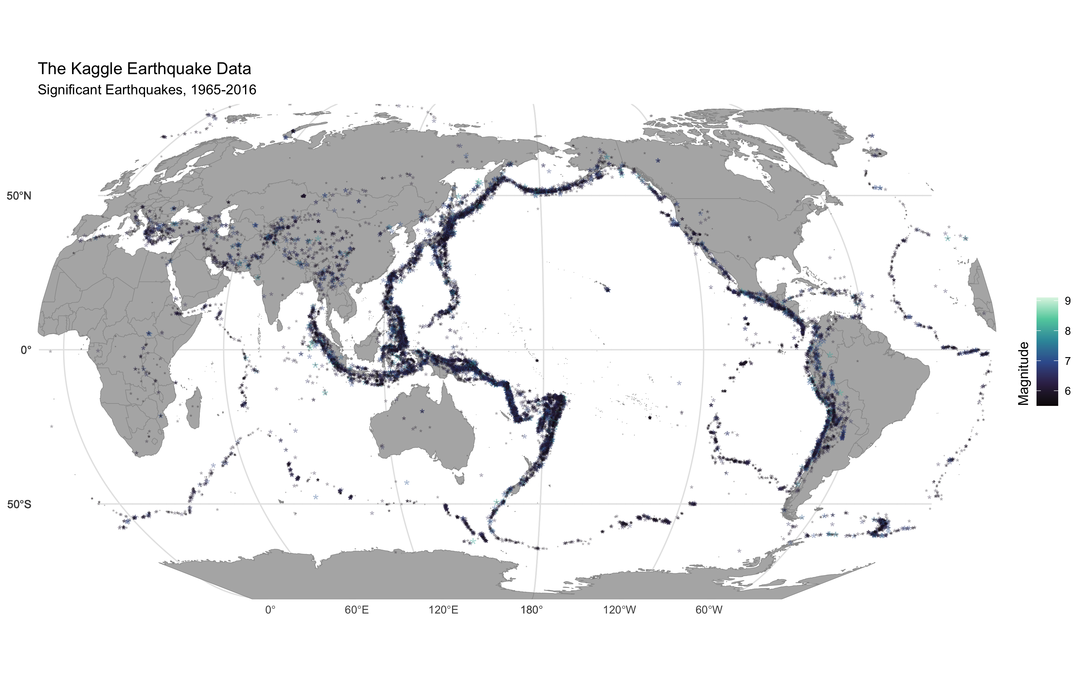
Reuse
Citation
BibTeX citation:
@online{smit,
  author = {Smit, A. J. and Smit, AJ},
  title = {Kaggle {Earthquake} {Database}},
  url = {https://tangledbank.netlify.app/pages/kaggle_earthquakes.html},
  langid = {en}
}
For attribution, please cite this work as:
Smit AJ, Smit A Kaggle Earthquake Database. https://tangledbank.netlify.app/pages/kaggle_earthquakes.html.