
flowchart TD
    A["Spatial Scale"] --> B["Global: Latitude"]
    A --> C["Regional: Rainfall Gradient"]
    A --> D["Local: Soil Moisture"]
Lecture 3. Ecological Gradients
NoteBCB743
This material must be reviewed by BCB743 students in Week 1 of Quantitative Ecology.
NoteBDC334 Lecture Transcript
Please see the BDC334 Lecture Transcript for the main content of all lectures.
TipThis Lecture Is Accompanied by the Following Labs
Environmental Gradients
This lecture links environmental variation to species distributions and community patterns across scales. We move from gradients and niches to species response models and neutral theory, then apply those ideas in global, regional, and local examples.
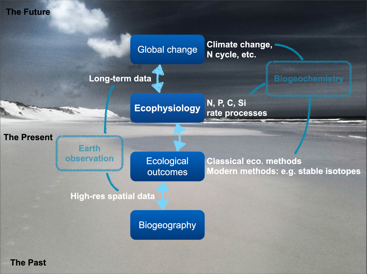
Environmental gradients are continuous changes in abiotic conditions across space or time that influence species performance and community composition. They link biodiversity outcomes, which we may measure as structure and function, to environmental properties (Figure 1). Biogeographical patterns help us discern how species distributions and community compositions vary in response to different environmental factors such as temperature, precipitation, and nutrient availability. Environmental drivers are variables that influence species distributions and ecosystem processes.
These gradients can be measured with Earth observation technologies, such as satellite remote sensing, alongside field observations and long-term environmental records.
As we move from present to future scenarios, long-term data allow us to use ecophysiological principles to understand how organisms and communities respond to changing environments. This includes climate change and major nutrient cycles (for example N, P, C, and Si). The key point is that gradients influence where species persist and how communities assemble.
In practice, ecologists work with several classes of gradients at once:
- Climatic gradients: temperature, rainfall, humidity, radiation, wind exposure.
- Edaphic gradients: soil texture, pH, salinity, nutrient availability, organic matter.
- Hydrological gradients: water depth, flow regime, inundation frequency, groundwater influence.
- Disturbance gradients: fire return interval, grazing intensity, storm exposure, anthropogenic disturbance.
Three broad-scale gradients are especially important because they organise patterns across terrestrial and marine systems:
- Elevational gradients (terrestrial): as elevation increases, temperature declines, oxygen partial pressure decreases, and vegetation often shifts in zones across slope and altitude.
- Depth gradients (marine): as depth increases, light declines, hydrostatic pressure rises, temperature often shifts, and community composition changes from shallow photic assemblages to deeper communities.
- Latitudinal gradients (global): poleward changes in temperature, seasonality, and radiation regimes are associated with large-scale turnover in biomes and species pools.
Elevation, depth, and latitude are proxy variables. Species respond to environmental conditions that covary with these gradients rather than to the geographic coordinates themselves.
These gradients operate across nested spatial scales:
- Continental scale: broad climate zones, major current systems, biome-level transitions.
- Landscape scale: topography, catchment position, land-cover mosaics, coast-to-inland shifts.
- Microhabitat scale: canopy vs open ground, rock crevices, tide pools, sediment patches.
Figure 2 summarises the global-to-local hierarchy that we will apply again in the examples later in this lecture.
They also vary through time, and that temporal structure matters for community assembly. Community assembly refers to the processes that determine which species occur together at a location:
- Seasonal gradients: within-year cycles in temperature, moisture, and productivity.
- Interannual gradients: year-to-year shifts linked to modes such as ENSO and regional circulation anomalies.
- Long-term climate change: multi-decadal directional changes in thermal and moisture regimes.
You can think of any location as having a “gradient fingerprint”: a specific combination of climatic, edaphic, hydrological, and disturbance conditions at a given time. Species sort along these fingerprints according to their tolerances, traits, and interactions.
Environmental gradients create variation in abiotic conditions. Species possess physiological tolerances to that variation. When species abundance is plotted against a gradient variable, the expected relationship often forms a unimodal response curve.
Environmental gradients create variation in conditions; Whittaker asked how species distributions respond to that variation.
To move from this broad idea to a usable ecological model, we next consider Whittaker’s contribution.
Whittaker and the Individualistic Hypothesis
Robert H. Whittaker (1920-1980) was instrumental in shaping our understanding of ecological gradients and their role in species community formation. He challenged the prevailing Clementsian view of communities as discrete, interdependent units, and proposed the “individualistic hypothesis” (Whittaker 1953). This hypothesis posits that species respond individually to environmental gradients, producing gradual shifts in community composition along those gradients.
Whittaker undertook extensive field research in diverse ecosystems, from the Great Smoky Mountains to the Siskiyou Mountains. This work provided strong empirical support for his hypothesis (Whittaker 1967). He also developed gradient analysis as a quantitative approach to studying species distributions along environmental gradients.
This perspective naturally leads to a testable species-level response model: the unimodal response curve.
The Unimodal Response Model
The unimodal model (sensu Whittaker 1967) provides a framework for understanding how species and communities are distributed along environmental gradients.
The model posits that the relationship between a species’ abundance (or biomass, frequency, or occurrence probability) and its position along a gradient follows a unimodal function. Abundance peaks at an optimum, where conditions are most suitable, and decreases as conditions deviate from that optimum in either direction.
This creates the characteristic bell-shaped response curve shown in Figure 3.
Show the code
library(coenocliner)
set.seed(666)
M <- 3                                     # number of species
ming <- 3.5                                # gradient minimum...
maxg <- 7                                  # ...and maximum
locs <- seq(ming, maxg, length = 100)      # gradient locations
opt  <- runif(M, min = ming, max = maxg)   # species optima
tol  <- rep(0.25, M)                       # species tolerances
h    <- ceiling(rlnorm(M, meanlog = 3))    # max abundances
pars <- cbind(opt = opt, tol = tol, h = h) # put in a matrix

mu <- coenocline(locs, responseModel = "gaussian", params = pars,
                 expectation = TRUE)

matplot(locs, mu, lty = "solid", type = "l", xlab = "pH", ylab = "Abundance")
The centre of the curve represents the environmental optimum, while the width of the curve represents the species’ tolerance range.
When species have different optima along the same gradient, their response curves overlap partially. As conditions change along the gradient, dominant species replace one another.
This model gives a simple mechanism for species sorting and turnover along gradients and underpins how we interpret patterns such as distance-decay and changes in community composition across, for example, elevation, rainfall, and temperature.
Why gradients matter for quantitative ecology
Gradient analysis is central to quantitative ecology because it underpins methods used later in this module:
- Ordination: summarising multivariate community patterns along dominant environmental axes.
- Species distribution models: estimating occurrence or abundance as a function of environmental predictors.
- Environmental distance metrics: quantifying how dissimilar sites are in abiotic conditions to explain turnover in community composition.
flowchart TD
    A["Environmental Gradient"] --> B["Species Response Curves"]
    B --> C["Community Composition"]
Figure 4 shows the lecture sequence in one view: abiotic variation shapes species responses, and aggregated responses shape community-level patterns.
The next step is to move from one gradient to many.
Multidimensional Gradient Space
In real ecosystems, species respond to multiple gradients at the same time: temperature, precipitation, soil chemistry, disturbance, hydrology, and others. Communities are therefore assembled in a multidimensional gradient space rather than along a single axis.
Within this space, each species has an optimum region and tolerance limits across several axes simultaneously. This is where coenoclines, coenoplanes, and coenospaces become useful analytical tools.
Coenoclines
A coenocline is a simplified representation of how a species (or a community attribute) changes along one environmental gradient. For example, rainfall often decreases from east to west across South Africa, and species abundances can shift accordingly.
Coenoclines are useful because they make species-environment relationships interpretable and comparable, especially when introducing gradient analysis.
Coenoplanes
When we model responses to two gradients simultaneously, we move from a line (coenocline) to a plane (coenoplane). This is often necessary because one-gradient explanations are usually incomplete in field systems.
For example, a species may respond jointly to temperature and moisture, with high abundance only where both are within a suitable range.
Coenospaces
When more than two gradients are considered, we work in a coenospace: a multidimensional representation of species and communities positioned by many interacting environmental variables.
For example, rainfall alone may explain some variation in plant communities (coenocline). When rainfall and temperature are analysed together, the response surface becomes a coenoplane. When additional variables such as soil nutrients and disturbance are included, the system becomes a coenospace.
Coenospaces provide the bridge between simple response curves and full community-assembly analyses in quantitative ecology.
Fundamental vs Realised Niches
The gradient-space framework connects directly to niche theory. The fundamental niche is the full set of abiotic conditions under which a species could persist in the absence of biotic constraints. The realised niche is the subset actually occupied once competition, predation, mutualisms, dispersal limits, and historical contingencies are considered.
A unimodal response curve can be interpreted as an expression of environmental tolerance. The set of conditions associated with positive population growth corresponds to the species’ niche.
This extends the pattern shown in Figure 4: environmental gradients shape species responses, and aggregated responses shape community composition.
In practice, this means observed species distributions are not explained by abiotic gradients alone. Biotic interactions can compress, shift, or occasionally expand realised occupancy relative to physiological potential.
Realised niches therefore represent the outcome of both environmental filtering and biotic interactions.
This sets up an important question: are communities primarily structured by niche differences, or can alternative mechanisms generate similar patterns?
Alternative Explanations of Community Structure
Niche-based gradient sorting is powerful, but it is not the only explanation for community structure. In many systems, stochastic processes, dispersal limitation, demographic drift, and historical contingency can also shape composition and abundance.
Niche-based explanations assume that species differ in their environmental responses. Neutral theory explores whether community patterns can arise even when species share similar ecological roles.
A complete interpretation of community patterns therefore compares deterministic niche models with stochastic alternatives.
Neutral theory
An important alternative (or complementary) framework is the Unified Neutral Theory of Biodiversity (UNTB). Neutral theory proposes that species in a trophically similar guild are functionally equivalent, and that relative abundances emerge largely from stochastic birth, death, dispersal, speciation, and extinction processes.
Neutral theory addresses a central question: how much of community structure can be generated by stochastic demographic and dispersal processes, even when species-level differences are weak or difficult to detect at the scale of observation?
Neutral theory tends to perform best in species-rich communities where ecological differences among species are difficult to detect at the scale of observation.
This differs from niche-based models, where species differ in tolerances and performance across environmental gradients. Niche models expect non-random sorting along gradients; neutral models expect patterns that can arise from ecological drift, dispersal limitation, and chance colonisation-extinction dynamics.
Both frameworks are useful, and each performs well under different conditions:
- Niche-based approaches tend to perform strongly when environmental heterogeneity is high and species trait differences are strongly expressed.
- Neutral approaches often perform well for broad-scale abundance distributions, species-area relationships, and communities where many species have similar measured performance.
- Many real systems require a blended interpretation where deterministic filtering and stochasticity both contribute.
The table below summarises the contrast:
| Framework | Mechanism | Expected pattern |
|---|---|---|
| Niche theory | Species respond differently to environmental variation and biotic interactions | Structured turnover and sorting along gradients |
| Neutral theory | Species are functionally equivalent within guilds; stochastic birth-death-dispersal dynamics dominate | Community composition shaped by drift, dispersal limitation, and chance |
Please consult:
Global Examples of Environmental Gradients
The same ecological mechanism can be traced across scales: global, regional, and local. We begin with a global example and then step down in extent.
At global scales, a classic pattern is latitude → temperature → biome transitions. Mean temperature and seasonality change with latitude, which contributes to broad biome structure (for example tropical forests, temperate systems, and polar or alpine environments). Global gradients also include rainfall belts linked to atmospheric circulation and marine thermal structure tied to major current systems.
These gradients influence species pools, productivity, and turnover, and they are measurable with global observation networks and long-term climate datasets. They provide the large-scale context within which regional and local community patterns emerge.
Regional Example: Southern Africa
At regional scale, Southern Africa provides a strong example of coupled terrestrial and marine gradients. Broadly, conditions are wetter in the east and drier in the west, and this pattern is linked to ocean-atmosphere coupling and topography.
The warm Agulhas system on the east coast contributes heat and moisture to the atmosphere, supporting higher rainfall and productivity in adjacent landscapes. Moving westward, moisture availability declines, rainfall decreases, and the dominant adaptive strategies of plants and animals shift accordingly.
This regional context helps explain why distinct biogeographic provinces occur across relatively short geographic distances.
Local Example: Cape Region Oceanic Transition
At local to subregional scales, a key transition zone occurs between Cape Point and Cape Agulhas (roughly 300 km), where Indian and Atlantic ocean influences interact. This creates a measurable transition in marine and coastal biota rather than a sharp, single boundary.
This interaction produces measurable turnover in marine communities, with warm-temperate assemblages transitioning to cold-temperate assemblages along the coast.
In this region, day-to-day weather variability is driven primarily by atmospheric pressure systems and frontal dynamics, while ocean currents provide slower but important background forcing at seasonal to interannual timescales. Together, these interacting drivers shape local environmental gradients and, in turn, community structure.
A detailed applied example is provided in the required reading on “Seaweeds in Two Oceans” (Smit et al. (2017)), where this transition is quantified in terms of community composition and biogeographic turnover.
Practical Integration with Labs 1-2 Workflow
The accompanying practicals translate gradient theory into data handling and distance-based comparison:
- Lab 1. Ecological Data: data structure, species/environment tables, and gradient-oriented ecological questions.
- Lab 2a. R & RStudio: reproducible setup for reading, transforming, and visualising gradient-linked data.
- Lab 2b. Environmental Distance: pairwise environmental distances used to represent separation among sites.
Use this workflow when moving from this lecture to the practicals:
- define the gradient hypothesis (e.g. community turnover increases along rainfall or temperature gradients),
- identify candidate gradient variables and scales (local, landscape, regional),
- prepare site × environment and site × species data in R,
- compute and inspect environmental distance structure among sites,
- interpret distances using the Lecture 3 framework (proxy gradients vs proximate drivers),
- compare distance patterns with observed compositional changes to evaluate mechanism plausibility.
Example Questions
NoteAnswer these yourself
Question 1. Environmental gradients and species responses
Environmental gradients organise biodiversity patterns across space and time.
Define an environmental gradient and explain why gradients are central to understanding species distributions. (4)
Describe Whittaker’s individualistic hypothesis and explain how it differs from earlier views of community organisation. (4)
Using the unimodal response model, explain how species abundances change along an environmental gradient. In your answer, interpret the meaning of the optimum and the tolerance range. (6)
Explain how overlapping unimodal response curves among species lead to gradual turnover in community composition along a gradient. (6)
Total: 20 marks
Purpose: tests the inferential chain gradient → species response → community pattern.
Question 2. Multidimensional gradients and niche structure
Species respond to multiple environmental variables simultaneously.
Explain the difference between a coenocline, coenoplane, and coenospace. (6)
Describe the difference between the fundamental niche and the realised niche. (4)
Explain how abiotic gradients and biotic interactions jointly determine the realised distribution of a species. (6)
Provide one ecological example in which two environmental gradients jointly determine species abundance or distribution. (4)
Total: 20 marks
Purpose: tests understanding of multidimensional gradients and niche interpretation.
Question 3. Community assembly across spatial scales
Ecological patterns often reflect processes operating at multiple spatial scales.
Describe a global environmental gradient and explain how it influences biome distribution. (5)
Using Southern Africa as an example, explain how regional environmental gradients influence biodiversity patterns. (7)
Describe the oceanographic transition between Cape Point and Cape Agulhas and explain how interacting environmental drivers influence local community structure. (4)
Compare niche-based explanations of community assembly with neutral theory. Under what ecological conditions might each framework provide useful explanations? (4)
Total: 20 marks
Purpose: evaluates the ability to integrate theory with global–regional–local examples.
References
Hubbell SP (2005) Neutral theory in community ecology and the hypothesis of functional equivalence. Functional ecology 19:166–172.
Hubbell SP (2011) The unified neutral theory of biodiversity and biogeography (MPB-32). Princeton University Press
Rosindell J, Hubbell SP, He F, Harmon LJ, Etienne RS (2012) The case for ecological neutral theory. Trends in ecology & evolution 27:203–208.
Smit AJ, Bolton JJ, Anderson RJ (2017) Seaweeds in two oceans: Beta-diversity. Frontiers in Marine Science 4:404.
Whittaker RH (1953) A consideration of climax theory: The climax as a population and pattern. Ecological monographs 23:41–78.
Whittaker RH (1967) Gradient analysis of vegetation.
Reuse
Citation
BibTeX citation:
@online{smit,_a._j.2024,
  author = {Smit, A. J.,},
  title = {Lecture 3. {Ecological} {Gradients}},
  date = {2024-07-22},
  url = {http://tangledbank.netlify.app/BDC334/Lec-03-gradients.html},
  langid = {en}
}
For attribution, please cite this work as:
Smit, A. J. (2024) Lecture 3. Ecological Gradients. http://tangledbank.netlify.app/BDC334/Lec-03-gradients.html.