---
date: last-modified
title: "24: A Complete Multivariate Analysis of the Doubs River"
format:
html:
code-link: false
code-fold: true
execute:
code-fold: true
---
```{r code-brewing-opts, echo=FALSE}
knitr::opts_chunk$set(
comment = "R>",
warning = FALSE,
message = FALSE,
fig.width = 4.5,
fig.height = 2.625,
out.width = "75%",
fig.asp = NULL, # control via width/height
dpi = 300
)
ggplot2::theme_set(
ggplot2::theme_bw(base_size = 8)
)
```
```{r code-setup-hidden}
#| echo: false
#| cache: false
library(tidyverse)
library(vegan)
library(viridis)
library(ggrepel)
library(patchwork)
library(gt)
# small helper used in inline text
fmt <- function(x, d = 2) formatC(x, format = "f", digits = d)
species_names <- c(
Cogo = "Bullhead",
Satr = "Brown trout",
Phph = "Minnow",
Babl = "Stone loach",
Thth = "Grayling",
Teso = "Souffia / Western vairone",
Chna = "Nase",
Pato = "Stone moroko",
Lele = "Sunbleak",
Sqce = "Chub",
Baba = "Barbel",
Albi = "Spirlin",
Gogo = "Gudgeon",
Eslu = "Pike",
Pefl = "Perch",
Rham = "Bitterling",
Legi = "Pumpkinseed",
Scer = "Rudd",
Cyca = "Crucian carp",
Titi = "Tench",
Abbr = "Common bream",
Icme = "Ide",
Gyce = "Ruffe",
Ruru = "Roach",
Blbj = "Silver bream",
Alal = "Bleak",
Anan = "Eel"
)
```
<!-- # Topic 24: A complete worked analysis -->
::: callout-tip
## **Material Required for This Chapter**
| Type | Name | Link |
| :--- | :--- | :--- |
| **Data** | The Doubs River data | [💾 `Doubs.RData`](../data/BCB743/NEwR-2ed_code_data/NeWR2-Data/Doubs.RData) |
| **Packages**| vegan, adespatial, betapart, mvabund, MASS, gt, leaflet | Install from CRAN before you start (see below) |
:::
::: {.callout-important appearance="simple"}
## Tasks to Complete in This Chapter
* Reproduce the workflow on the Doubs data, then repeat it on a dataset of your own choosing.
:::
Throughout the module the Doubs River fish survey was used as an example, but we examined the dataset one method at a time. Here I apply the whole suite of functions to it at once, from the first unconstrained ordination to methods from outside the core syllabus. So, this is a synthesis chapter. The interest is where the methods agree, where they diverge, and what each one adds that the others miss.
The Doubs analyses repeatedly recover the longitudinal river continuum, but the more revealing ecological structure is seen where that continuum breaks down. The chapter also shows that statistical procedures can summarise pattern efficiently, while causal insights must come from ecological interpretation.
Spatial structure is represented through Moran eigenvector maps computed by `dbmem()`, also new to the module. The data-driven variable selection of `ordiR2step()` is then compared to a theory-driven alternative, which is a way of thinking rather than a function call. Everything else you have seen before, and I cross-reference the chapter where you have seen it.
## Study Region
The Doubs River rises in the Jura Mountains near Mouthe, follows the French-Swiss border for part of its upper and middle course, then turns west and south-west through Besancon and Dole before joining the Saone. The map in @fig-doubs-region is a geographic orientation map of the river region, not a plot of the sampling coordinates. The `spa` object in `Doubs.RData` contains local planar coordinates, so I use it later for spatial modelling rather than placing those points directly on a web map.
```{r fig-doubs-region}
#| label: fig-doubs-region
#| fig-cap: "Topographic overview of the Doubs River region. The blue line is an approximate course drawn through major river landmarks to orient the study region."
#| out-width: "100%"
doubs_landmarks <- tibble::tribble(
  ~place                , ~reach                      , ~lon  , ~lat   ,
  "Mouthe"              , "Source region"             , 6.193 , 46.709 ,
  "Pontarlier"          , "Upper Doubs"               , 6.355 , 46.904 ,
  "Morteau"             , "Upper border reach"        , 6.607 , 47.057 ,
  "Goumois"             , "French-Swiss border reach" , 6.953 , 47.263 ,
  "Besancon"            , "Middle Doubs"              , 6.025 , 47.238 ,
  "Dole"                , "Lower Doubs"               , 5.489 , 47.092 ,
  "Verdun-sur-le-Doubs" , "Confluence with the Saone" , 5.023 , 46.897
)

leaflet::leaflet(doubs_landmarks, height = "430px") |>
  leaflet::addProviderTiles(
    leaflet::providers$Esri.WorldTopoMap,
    options = leaflet::providerTileOptions(opacity = 0.95)
  ) |>
  leaflet::addPolylines(
    lng = ~lon,
    lat = ~lat,
    color = "#2166ac",
    weight = 4,
    opacity = 0.9,
    label = "Approximate Doubs River course"
  ) |>
  leaflet::addCircleMarkers(
    lng = ~lon,
    lat = ~lat,
    radius = 5,
    stroke = TRUE,
    weight = 1,
    color = "#111111",
    fillColor = "#b2182b",
    fillOpacity = 0.9,
    popup = ~ paste0("<strong>", place, "</strong><br>", reach)
  ) |>
  leaflet::addLabelOnlyMarkers(
    lng = ~lon,
    lat = ~lat,
    label = ~place,
    labelOptions = leaflet::labelOptions(
      noHide = TRUE,
      direction = "auto",
      textOnly = TRUE,
      offset = c(6, 0),
      style = list(
        "font-size" = "11px",
        "font-weight" = "600",
        "text-shadow" = "0 0 3px #ffffff"
      )
    )
  ) |>
  leaflet::fitBounds(
    lng1 = 4.85,
    lat1 = 46.55,
    lng2 = 7.10,
    lat2 = 47.45
  ) |>
  leaflet::addScaleBar(position = "bottomleft")
```
::: callout-note
## Packages you may need to install
Beyond **vegan** and the **tidyverse**, this chapter uses **leaflet** (interactive maps), **adespatial** (spatial eigenvectors and beta-diversity contributions), **betapart** (turnover and nestedness), **mvabund** (model-based multivariate GLMs), **MASS** (negative-binomial GLMs), and **gt** (tables). Install any you are missing with `install.packages(c("leaflet", "adespatial", "betapart", "mvabund", "gt"))`. **MASS** ships with R.
:::
## Set-up the Analysis Environment
```{r code-libraries}
#| cache: false
library(tidyverse)
library(vegan)
library(viridis)
library(ggrepel)
library(patchwork)
library(gt) # publication-quality tables
```
I load the Doubs data. The file holds five objects, of which I use the fish abundances (`spe`), the environmental table (`env`), and the spatial coordinates (`spa`).
```{r code-load-data}
load(here::here(
  "data",
  "BCB743",
  "NEwR-2ed_code_data",
  "NEwR2-Data",
  "Doubs.RData"
))
dim(spe)
dim(env)
dim(spa)
```
Site 8 has no fish, so it has no compositional information and breaks the $\chi^2$ and Bray-Curtis geometries (you have seen this problem in the [CA chapter](CA.qmd)). I drop it from the species-based analyses and keep a matched set of 29 sites. The environmental PCA can use all 30 rows, since it does not depend on the fish. I also standardise the environmental variables to zero mean and unit variance, so that variables measured on different scales (metres of altitude against milligrams of nitrate) contribute comparably.
```{r code-prep-data}
keep <- rowSums(spe) > 0 # site 8 is the only FALSE
spe <- spe[keep, ]
env_matched <- env[keep, ]
spa <- spa[keep, ]

E <- as.data.frame(scale(env_matched)) # standardised predictors
spe_hel <- decostand(spe, "hellinger") # Hellinger transform for RDA
site_dfs <- env_matched$dfs # distance from source, the river order
```
```{r code-gt-helper}
#| echo: false
gt_doubs <- function(df, note = NULL) {
g <- df |>
gt() |>
tab_options(
table.font.size = px(13),
column_labels.font.weight = "bold",
column_labels.background.color = "#f2f2f2",
data_row.padding = px(4),
heading.align = "left",
table.border.top.width = px(2),
table.border.top.color = "#111111",
table.border.bottom.width = px(2),
table.border.bottom.color = "#111111",
source_notes.font.size = px(10)
) |>
opt_horizontal_padding(1.5)
if (!is.null(note)) {
g <- g |> tab_source_note(md(note))
}
g
}
```
The first summary already shows the main structure of the river. Each environmental variable is reduced to its range and its correlation with distance from source, so the table asks, which measurements are really tracking the downstream axis?
```{r tbl-env-summary}
#| label: tbl-env-summary
#| tbl-cap: "Environmental variables of the Doubs River, their range across the 30 sites, and their Pearson correlation with distance from source."
var_labels <- c(
  dfs = "Distance from source",
  ele = "Altitude",
  slo = "Channel slope",
  dis = "Flow rate",
  pH = "pH",
  har = "Water hardness",
  pho = "Phosphate",
  nit = "Nitrate",
  amm = "Ammonium",
  oxy = "Dissolved oxygen",
  bod = "Biological oxygen demand"
)

env_summary <- tibble(
  Code = names(env),
  Variable = var_labels[names(env)],
  Minimum = map_dbl(env, min),
  Median = map_dbl(env, median),
  Maximum = map_dbl(env, max),
  r_dfs = map_dbl(env, ~ cor(.x, env$dfs))
)

env_summary |>
  gt_doubs(
    note = "Source: `Doubs.RData`. *r* with dfs computed across all 30 sites."
  ) |>
  cols_label(Code = "", r_dfs = "r with dfs") |>
  fmt_number(columns = c(Minimum, Median, Maximum, r_dfs), decimals = 2) |>
  data_color(
    columns = r_dfs,
    palette = c("#2166ac", "#f7f7f7", "#b2182b"),
    domain = c(-1, 1)
  )
```
The heatmap column shows that distance from source, flow, hardness, nitrate, and phosphate rise downstream; altitude, slope, and oxygen fall; pH barely moves. The eleven variables all views of one downstream integration of geomorphology and chemistry rather; they don't seem to function as independent measurements. The rest of the chapter traces this gradient (and exceptions) through the fish.
## The Dominant Gradient: Unconstrained Ordinations
The first check is whether the dominant gradient is robust to the geometry of the analysis. Applying the ordination workflow developed earlier in the module gives four first axes to compare: environmental PCA, species CA, Bray-Curtis PCoA, and Bray-Curtis nMDS.
```{r code-unconstrained}
set.seed(743)
env_pca <- rda(env, scale = TRUE) # all 30 sites
spe_ca <- cca(spe) # correspondence analysis
spe_dca <- decorana(spe) # detrended CA
spe_pcoa <- capscale(spe ~ 1, distance = "bray") # PCoA on Bray-Curtis
spe_nmds <- metaMDS(
  spe,
  distance = "bray",
  trace = 0,
  autotransform = FALSE,
  trymax = 100
) # nMDS
```
The two-dimensional configurations in @fig-unconstrained show what those
first-axis summaries compress. Sites are coloured by their distance from the
source, so a smooth colour transition across an ordination indicates recovery
of the longitudinal river gradient. DCA is included here because its axis
length is used below to diagnose the long species-turnover gradient, even
though it is not part of the four-method correlation comparison.
```{r fig-unconstrained}
#| label: fig-unconstrained
#| fig-cap: "Site configurations from each unconstrained ordination. Numbers identify sampling sites and colour shows distance from the source. PCA uses all 30 sites; the species ordinations exclude fishless site 8."
#| fig-width: 8
#| fig-height: 10.8
#| out-width: "100%"
#| code-fold: true
site_ordination_panel <- function(
  ord,
  title,
  dfs,
  labels,
  axis_names = NULL,
  scaling = 1
) {
  xy <- as.data.frame(scores(
    ord,
    display = "sites",
    choices = 1:2,
    scaling = scaling
  ))
  names(xy)[1:2] <- c("Axis1", "Axis2")
  xy$dfs <- dfs
  xy$site <- labels

  if (is.null(axis_names)) {
    axis_names <- colnames(scores(
      ord,
      display = "sites",
      choices = 1:2,
      scaling = scaling
    ))[1:2]
  }

  ggplot(xy, aes(Axis1, Axis2, colour = dfs)) +
    geom_hline(yintercept = 0, colour = "grey88", linewidth = 0.3) +
    geom_vline(xintercept = 0, colour = "grey88", linewidth = 0.3) +
    geom_point(size = 1.7) +
    geom_text_repel(
      aes(label = site),
      size = 2.2,
      max.overlaps = Inf,
      min.segment.length = 0,
      show.legend = FALSE
    ) +
    scale_colour_viridis_c(option = "viridis", name = "Distance\nfrom source") +
    labs(title = title, x = axis_names[1], y = axis_names[2]) +
    theme(
      plot.title = element_text(face = "bold", size = 9),
      legend.position = "right"
    )
}

p_pca <- site_ordination_panel(
  env_pca,
  "Environmental PCA",
  env$dfs,
  seq_len(nrow(env))
)
p_ca <- site_ordination_panel(
  spe_ca,
  "Correspondence analysis",
  site_dfs,
  rownames(spe)
)
p_dca <- site_ordination_panel(
  spe_dca,
  "Detrended correspondence analysis",
  site_dfs,
  rownames(spe)
)
p_pcoa <- site_ordination_panel(
  spe_pcoa,
  "Bray-Curtis PCoA",
  site_dfs,
  rownames(spe)
)

nmds_xy <- as.data.frame(spe_nmds$points[, 1:2])
names(nmds_xy) <- c("Axis1", "Axis2")
nmds_xy$dfs <- site_dfs
nmds_xy$site <- rownames(spe)
p_nmds <- ggplot(nmds_xy, aes(Axis1, Axis2, colour = dfs)) +
  geom_hline(yintercept = 0, colour = "grey88", linewidth = 0.3) +
  geom_vline(xintercept = 0, colour = "grey88", linewidth = 0.3) +
  geom_point(size = 1.7) +
  geom_text_repel(
    aes(label = site),
    size = 2.2,
    max.overlaps = Inf,
    min.segment.length = 0,
    show.legend = FALSE
  ) +
  scale_colour_viridis_c(option = "viridis", name = "Distance\nfrom source") +
  labs(
    title = paste0("Bray-Curtis nMDS (stress = ", fmt(spe_nmds$stress, 3), ")"),
    x = "NMDS1",
    y = "NMDS2"
  ) +
  theme(
    plot.title = element_text(face = "bold", size = 9),
    legend.position = "right"
  )

wrap_plots(p_pca, p_ca, p_dca, p_pcoa, p_nmds, ncol = 2) +
  plot_layout(guides = "collect") &
  theme(legend.position = "bottom")
```
The test: a real river gradient should align with distance from source no matter which geometry produced the axis. Because ordination signs are arbitrary, I compare absolute correlations.
```{r code-gradient-align}
first_axis <- function(ord, dfs) {
  s <- scores(ord, display = "sites", choices = 1)
  abs(cor(as.numeric(s), dfs))
}

align <- tibble(
  Ordination = c("PCA (PC1)", "CA (CA1)", "PCoA (MDS1)", "nMDS (NMDS1)"),
  r_with_dfs = c(
    abs(cor(scores(env_pca, display = "sites", choices = 1)[keep], site_dfs)),
    first_axis(spe_ca, site_dfs),
    first_axis(spe_pcoa, site_dfs),
    abs(cor(spe_nmds$points[, 1], site_dfs))
  )
)

# precomputed for inline use (avoids calling vegan functions in inline text)
dca_len <- diff(range(scores(spe_dca, display = "sites", choices = 1)))
```
```{r tbl-align}
#| label: tbl-align
#| tbl-cap: "Correlation of each unconstrained ordination's first axis with distance from source."
align |>
  gt_doubs(
    note = "Absolute Pearson correlation; ordination axis signs are arbitrary."
  ) |>
  cols_label(r_with_dfs = "|r| with dfs") |>
  fmt_number(columns = r_with_dfs, decimals = 3) |>
  data_color(columns = r_with_dfs, palette = "Blues", domain = c(0, 1))
```
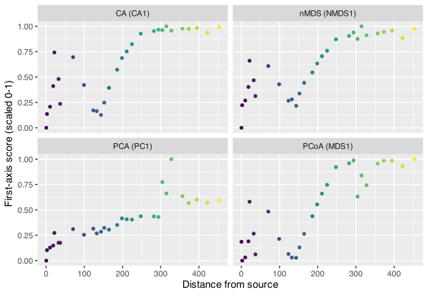
The four correlations range from about 0.81 to 0.85 (@tbl-align). An axis extracted from the environmental table alone, an axis extracted from the fish alone under the $\chi^2$ metric, and two axes extracted from Bray-Curtis dissimilarity all reconstruct the same upstream-to-downstream order. So, I confirm that the dominant structure is a property of the river rather than of any one method. @fig-align shows the same pattern.
```{r fig-align}
#| label: fig-align
#| fig-cap: "First-axis site scores of the four unconstrained ordinations against distance from source. Each ordination recovers the same monotonic river gradient. Scores are scaled to a common range and oriented to increase downstream."
#| fig-width: 6.5
#| fig-height: 4.5
#| code-fold: true
rescale01 <- function(x) {
  x <- x * sign(cor(x, site_dfs)) # orient to increase with dfs
  (x - min(x)) / (max(x) - min(x))
}

axis_scores <- tibble(
  dfs = site_dfs,
  `PCA (PC1)` = rescale01(scores(env_pca, display = "sites", choices = 1)[
    keep
  ]),
  `CA (CA1)` = rescale01(as.numeric(scores(
    spe_ca,
    display = "sites",
    choices = 1
  ))),
  `PCoA (MDS1)` = rescale01(as.numeric(scores(
    spe_pcoa,
    display = "sites",
    choices = 1
  ))),
  `nMDS (NMDS1)` = rescale01(spe_nmds$points[, 1])
) |>
  pivot_longer(-dfs, names_to = "Ordination", values_to = "score")

ggplot(axis_scores, aes(dfs, score, colour = dfs)) +
  geom_point(size = 1.3) +
  facet_wrap(~Ordination) +
  scale_colour_viridis_c(guide = "none") +
  labs(x = "Distance from source", y = "First-axis score (scaled 0-1)")
```
DCA's first-axis length, `r fmt(dca_len)` standard-deviation units, is long, which means the fish turn over almost completely from source to mouth. A long gradient is why CA and PCA of these species show an arch, and why the distance-based methods, which do not force a linear response, describe the community more faithfully. That is the reasoning you'll have seen in the [DCA](DCA.qmd) and [PCoA](PCoA.qmd) chapters, and I take it as given here.
## Constrained Ordination and Variable Selection
The unconstrained methods describe the pattern; the constrained methods ask whether the measured environment explains it. I run the three familiar constrained approaches in parallel, RDA, CCA, and db-RDA, and compare the variables retained by forward selection.
```{r code-constrained}
set.seed(743)

# RDA (linear, Hellinger)
rda_full <- rda(spe_hel ~ ., data = E)
rda_0 <- rda(spe_hel ~ 1, data = E)
rda_sel <- ordiR2step(
  rda_0,
  scope = formula(rda_full),
  R2scope = TRUE,
  trace = FALSE
)

# CCA (unimodal, chi-square)
cca_full <- cca(spe ~ ., data = E)
cca_0 <- cca(spe ~ 1, data = E)
cca_sel <- ordiR2step(
  cca_0,
  scope = formula(cca_full),
  R2scope = TRUE,
  trace = FALSE
)

# db-RDA (any dissimilarity, here Bray-Curtis)
dbrda_full <- capscale(spe ~ ., data = E, distance = "bray")
dbrda_0 <- capscale(spe ~ 1, data = E, distance = "bray")
dbrda_sel <- ordiR2step(
  dbrda_0,
  scope = formula(dbrda_full),
  R2scope = TRUE,
  trace = FALSE
)
```
The selected ordinations are shown in @fig-constrained. Here the arrows are the
predictors retained by forward selection, and the sites are again coloured by
distance from source. Arrow direction shows increasing values; arrow length is
scaled within each panel for legibility and should not be compared across
methods.
```{r fig-constrained}
#| label: fig-constrained
#| fig-cap: "Selected RDA, CCA, and Bray-Curtis db-RDA ordinations. Points are sampling sites, colour indicates distance from the source, and arrows show the environmental variables retained by forward selection."
#| fig-width: 9
#| fig-height: 3.7
#| out-width: "100%"
#| code-fold: true
constrained_panel <- function(ord, title) {
  site_xy <- as.data.frame(scores(
    ord,
    display = "sites",
    choices = 1:2,
    scaling = 2
  ))
  names(site_xy)[1:2] <- c("Axis1", "Axis2")
  site_xy$dfs <- site_dfs
  site_xy$site <- rownames(spe)

  bp_xy <- as.data.frame(scores(
    ord,
    display = "bp",
    choices = 1:2,
    scaling = 2
  ))
  names(bp_xy)[1:2] <- c("Axis1", "Axis2")
  bp_xy$variable <- rownames(bp_xy)

  arrow_multiplier <- 0.75 *
    min(
      diff(range(site_xy$Axis1)) / diff(range(bp_xy$Axis1)),
      diff(range(site_xy$Axis2)) / diff(range(bp_xy$Axis2))
    )
  bp_xy <- bp_xy |>
    mutate(
      Axis1 = Axis1 * arrow_multiplier,
      Axis2 = Axis2 * arrow_multiplier
    )

  axis_names <- colnames(scores(
    ord,
    display = "sites",
    choices = 1:2,
    scaling = 2
  ))[1:2]

  ggplot(site_xy, aes(Axis1, Axis2)) +
    geom_hline(yintercept = 0, colour = "grey88", linewidth = 0.3) +
    geom_vline(xintercept = 0, colour = "grey88", linewidth = 0.3) +
    geom_point(aes(colour = dfs), size = 1.7) +
    geom_segment(
      data = bp_xy,
      aes(x = 0, y = 0, xend = Axis1, yend = Axis2),
      inherit.aes = FALSE,
      arrow = arrow(length = unit(1.5, "mm")),
      colour = "#b2182b",
      linewidth = 0.45
    ) +
    geom_text_repel(
      data = bp_xy,
      aes(Axis1, Axis2, label = variable),
      inherit.aes = FALSE,
      colour = "#b2182b",
      fontface = "bold",
      size = 2.5,
      min.segment.length = 0
    ) +
    scale_colour_viridis_c(option = "viridis", name = "Distance\nfrom source") +
    labs(title = title, x = axis_names[1], y = axis_names[2]) +
    theme(plot.title = element_text(face = "bold", size = 9))
}

wrap_plots(
  constrained_panel(rda_sel, "Selected RDA"),
  constrained_panel(cca_sel, "Selected CCA"),
  constrained_panel(dbrda_sel, "Selected db-RDA"),
  nrow = 1
) +
  plot_layout(guides = "collect") &
  theme(legend.position = "bottom")
```
The full models have severe collinearity, with VIFs in the hundreds because the river variables are correlated together. Forward selection reduces this redundancy to interpretable levels. The table compares the selected predictors, adjusted $R^2$, and the maximum VIF before and after selection.
```{r code-model-summary}
#| echo: false
selected_vars <- function(mod) {
paste(all.vars(formula(mod))[-1], collapse = ", ")
}
set.seed(743)
model_summary <- tibble(
Model = c("RDA", "CCA", "db-RDA"),
Predictors = c(
selected_vars(rda_sel),
selected_vars(cca_sel),
selected_vars(dbrda_sel)
),
adjR2 = c(
RsquareAdj(rda_sel)$adj.r.squared,
RsquareAdj(cca_sel)$adj.r.squared,
RsquareAdj(dbrda_sel)$adj.r.squared
),
maxVIF_full = c(
max(vif.cca(rda_full)),
max(vif.cca(cca_full)),
max(vif.cca(dbrda_full))
),
maxVIF_sel = c(
max(vif.cca(rda_sel)),
max(vif.cca(cca_sel)),
max(vif.cca(dbrda_sel))
)
)
```
```{r tbl-model-summary}
#| label: tbl-model-summary
#| tbl-cap: "The three constrained models after forward selection, with adjusted R-squared and the maximum VIF before and after selection."
model_summary |>
  gt_doubs(
    note = "Forward selection by `ordiR2step()`; VIF from `vif.cca()`."
  ) |>
  cols_label(
    adjR2 = "adj. R²",
    maxVIF_full = "max VIF (full)",
    maxVIF_sel = "max VIF (selected)"
  ) |>
  fmt_number(columns = adjR2, decimals = 3) |>
  fmt_number(columns = c(maxVIF_full, maxVIF_sel), decimals = 1) |>
  tab_style(
    style = cell_fill(color = "#eef6ff"),
    locations = cells_body(rows = Model == "db-RDA")
  )
```
The three models converge (@tbl-model-summary). Each keeps a longitudinal-position variable (a proxy variable), `dfs` or `ele` (elevation, the altitude proxy in this dataset), together with `oxy` and a marker of organic loading. The maximum VIF falls from the hundreds in the full models to single digits after selection. The models agree that about half of the community variation is captured by three correlated descriptors of river position. The convergence has more weight than the small differences between the models.
Notice a common theme that now runs through much of multivariate ecology: permutation tests. RDA, CCA, db-RDA, Mantel tests, LCBD tests, and manyGLM resampling all use permutations or resampling to check whether the observed structure is stronger than expected after rearranging the data under an appropriate null model. The details differ, but the logic is the same. We are not usually relying on closed-form normal theory; we are asking whether the community pattern survives comparison with many reordered versions of itself.
### Data-driven and theory-driven variable selection {#sec-selection}
This is an important part in the chapter, because the selected variables are easy to over-interpret. Forward selection is a statistical procedure so ecological theory is not involved anywhere. It keeps whichever variables most raise adjusted $R^2$, and in these data that is `dfs` with `oxy` and `bod`. A mechanistic account of the same river starts elsewhere. Position sets the physical foundation, since altitude and distance from source drive temperature, slope, and discharge. Land use then enriches the water with dissolved inorganic nitrogen (DIN, namely nitrate plus ammonium) and phosphate. This nutrient load drives primary production and the supply of degradable organic matter, which raises biological oxygen demand, and the respiration that follows draws down oxygen. In this chain nutrients are the upstream driver and oxygen is a downstream consequence.
So if we want a *cause* rather than a *correlate*, we might prefer a nutrient variable over oxygen. I can put that intuition to a direct test by fitting the candidate models by hand and comparing them, which is a good habit whenever a stepwise algorithm returns a set of variables.
```{r code-theory-compare}
candidates <- list(
  "Forward-selected" = spe_hel ~ dfs + oxy + bod,
  "Position only" = spe_hel ~ dfs,
  "Position + nitrate" = spe_hel ~ dfs + nit,
  "Nutrient loading" = spe_hel ~ ele + nit + amm,
  "Nutrient + phosphate" = spe_hel ~ ele + nit + pho
)

theory_compare <- imap_dfr(candidates, function(f, nm) {
  m <- rda(f, data = E)
  tibble(
    Model = nm,
    Predictors = paste(all.vars(f)[-1], collapse = ", "),
    adjR2 = RsquareAdj(m)$adj.r.squared,
    maxVIF = max(vif.cca(m))
  )
})
```
```{r tbl-theory-compare}
#| label: tbl-theory-compare
#| tbl-cap: "Data-driven and theory-driven candidate models, all fitted as Hellinger RDA, with adjusted R-squared and the maximum VIF of each predictor set."
theory_compare |>
  gt_doubs(
    note = "adj. R² measures fit; max VIF measures residual collinearity."
  ) |>
  cols_label(adjR2 = "adj. R²", maxVIF = "max VIF") |>
  fmt_number(columns = adjR2, decimals = 3) |>
  fmt_number(columns = maxVIF, decimals = 2) |>
  tab_style(
    style = cell_text(weight = "bold"),
    locations = cells_body(columns = adjR2, rows = adjR2 == max(adjR2))
  )
```
Distance from source alone reaches adjusted $R^2 \approx 0.37$ (@tbl-theory-compare). Adding nitrate raises it only to about 0.39, whereas adding oxygen and biological oxygen demand increases it to 0.54. The nutrient-loading models stabilise near 0.39 as well. Dropping the oxygen pair forfeits about 0.15 of adjusted $R^2$, a difference too large to ignore. Why does the nutrient model explain so much less, if nutrients are meant to drive the oxygen? The correlation heatmap explains why.
```{r tbl-enrich-cor}
#| label: tbl-enrich-cor
#| tbl-cap: "Pearson correlations among distance from source and the enrichment variables across the 29 matched sites."
enrich_vars <- c("dfs", "oxy", "bod", "nit", "amm", "pho")
cor_tab <- cor(env_matched[, enrich_vars]) |>
  round(2) |>
  as.data.frame() |>
  rownames_to_column("Variable")

cor_tab |>
  gt_doubs(
    note = "Pearson correlations; cells shaded from blue (-1) to red (+1)."
  ) |>
  fmt_number(columns = all_of(enrich_vars), decimals = 2) |>
  data_color(
    columns = all_of(enrich_vars),
    palette = c("#2166ac", "#f7f7f7", "#b2182b"),
    domain = c(-1, 1)
  )
```
Along the clean part of the continuum the enrichment variables are correlated, with several pairwise correlations above 0.7 in absolute value (@tbl-enrich-cor), so any one can replace others and the choice among them is interpretive. The exception is where the ecology becomes interesting. Nitrate rises almost monotonically with distance from source ($r \approx 0.74$) and tracks the continuum, whereas oxygen and BOD decouple from it at the mid-river reach near sites 23 to 25, where oxygen falls to 4 to 6 mg L^-1^ and BOD exceeds 12 mg L^-1^. Forward selection retains oxygen and BOD precisely because they have that local oxygen sag, which a position or nitrate model cannot reproduce.
The interpretation is therefore a bit more complicated than it previously emerged in the earlier chapters. For a management question about nutrient control, DIN is the defensible predictor, and it loses little fit over the continuum. For describing the community that is actually present, oxygen is more than a proxy, and near the polluted sites it is a proximate stressor with a signal of its own. Statistical selection cannot arbitrate between these interpretations, because the variables are collinear over most of the river and diverge only at a handful of sites. The choice is an ecological judgement informed by the correlation structure, not an output of the algorithm. This is what the [constrained ordination chapter](constrained_ordination.qmd) means by *explanation is not causation*.
## Beyond the Core Ordination Methods
In the remaining methods I do not revisit the ordination workflow. I ask additional ecological question about the same result, viz., how much is space, where does the continuum break, is the change replacement or loss, which sites are distinctive, and do species-level models tell the same story?
### Separating environment from space with variation partitioning
Sites that are far downstream are also far along the channel, so environment and space are structurally confounded. Variation partitioning is useful here because the shared fraction is itself ecological evidence: in a single river, environmental change and geographic position are partly the same thing.
```{r code-varpart}
space_poly <- with(
  as.data.frame(scale(spa)),
  data.frame(X, Y, X2 = X^2, Y2 = Y^2, XY = X * Y)
)
E_sel <- E[, all.vars(formula(dbrda_sel))[-1]] # the db-RDA predictors

vp <- varpart(spe_hel, E_sel, space_poly)
vp
```
```{r fig-varpart}
#| label: fig-varpart
#| fig-cap: "Venn partition of Hellinger-transformed fish composition between the selected environmental predictors and polynomial spatial position. Values are adjusted R-squared for each fraction."
#| fig-width: 4.5
#| fig-height: 4.5
#| code-fold: true
plot(
  vp,
  bg = c("#8ecae6", "#ffb703"),
  Xnames = c("Environment", "Space"),
  digits = 2,
  cutoff = -Inf
)
```
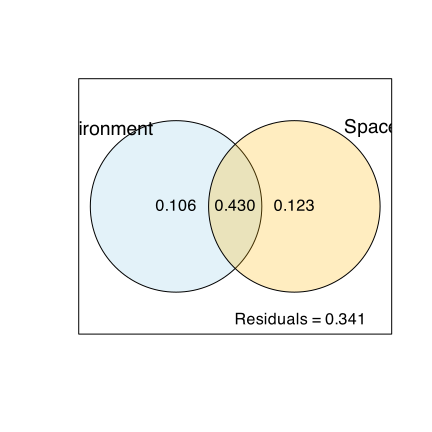
The pure environmental and pure spatial fractions are both small (adjusted $R^2 \approx 0.11$ and $0.12$), while the shared fraction reaches about 0.43 (@fig-varpart). Most of the explained variation cannot be assigned to environment or to space alone, because in a single river the two are the same axis viewed twice. A large shared fraction here is ecological information, not a nuisance to be removed.
### Spatial structure at multiple scales with MEM
Variation partitioning treats space as a smooth trend. Moran eigenvector maps (MEMs) are more flexible and are new in this chapter. They describe spatial structure at multiple scales, from a broad upstream-to-downstream pattern to finer alternation among neighbouring reaches.
```{r code-mem}
library(adespatial)

mem <- dbmem(spa, silent = TRUE) # Moran eigenvector maps from coordinates
mem_df <- as.data.frame(mem)

set.seed(743)
mem_full <- rda(spe_hel ~ ., data = mem_df)
mem_0 <- rda(spe_hel ~ 1, data = mem_df)
mem_sel <- ordiR2step(
  mem_0,
  scope = formula(mem_full),
  R2scope = TRUE,
  trace = FALSE
)

mem_vars <- selected_vars(mem_sel)
mem_r2 <- RsquareAdj(mem_sel)$adj.r.squared
mem_vars
mem_r2
```
@fig-mem-ordination displays the spatial RDA itself. The arrows show the
selected spatial eigenvectors, while the colour gradient reveals whether their
combined configuration represents the broad river continuum or finer-scale
departures from it.
```{r fig-mem-ordination}
#| label: fig-mem-ordination
#| fig-cap: "RDA of fish composition constrained by the forward-selected Moran eigenvector maps. Points are sampling sites, colour indicates distance from the source, and arrows show the selected spatial eigenvectors."
#| fig-width: 5.5
#| fig-height: 4.2
#| code-fold: true
constrained_panel(mem_sel, "Selected MEM-based RDA")
```
Forward selection keeps `r mem_vars` and reaches an adjusted $R^2$ of about `r fmt(mem_r2)`. The fish assemblage is spatially structured, and the broad-scale MEMs have the same longitudinal signal as distance from source. MEMs do not implicate an environmental cause. They quantify the scale at which structure exists, which is a useful addition to the variation partitioning above and a standard starting point to spatial community ecology.
### Comparing whole matrices with Mantel tests
A Mantel test is the matrix-level counterpart of the previous section. It asks whether sites that are environmentally or geographically far apart are also far apart in fish composition, without first reducing the matrices to ordination axes.
```{r code-mantel}
D_comm <- vegdist(spe, method = "bray")
D_env <- dist(E)
D_geo <- dist(spa)

set.seed(743)
mantel_tab <- tibble(
  Comparison = c(
    "Community vs environment",
    "Community vs geography",
    "Community vs environment | geography",
    "Community vs geography | environment"
  ),
  r = c(
    mantel(D_comm, D_env)$statistic,
    mantel(D_comm, D_geo)$statistic,
    mantel.partial(D_comm, D_env, D_geo)$statistic,
    mantel.partial(D_comm, D_geo, D_env)$statistic
  ),
  p = c(
    mantel(D_comm, D_env)$signif,
    mantel(D_comm, D_geo)$signif,
    mantel.partial(D_comm, D_env, D_geo)$signif,
    mantel.partial(D_comm, D_geo, D_env)$signif
  )
)
```
```{r tbl-mantel}
#| label: tbl-mantel
#| tbl-cap: "Mantel and partial Mantel correlations among the fish, environmental, and geographic distance matrices."
mantel_tab |>
  gt_doubs(
    note = "Mantel *r* with 999 permutations; the vertical bar denotes 'holding constant'."
  ) |>
  fmt_number(columns = r, decimals = 3) |>
  fmt_number(columns = p, decimals = 3) |>
  tab_style(
    style = cell_text(color = "#b2182b", weight = "bold"),
    locations = cells_body(columns = p, rows = p <= 0.05)
  )
```
The environment is much the stronger match ($r \approx 0.61$ against $0.32$ for geography), and it survives conditioning on space ($r \approx 0.56$) far better than space survives conditioning on environment ($r \approx 0.18$) (@tbl-mantel). This agrees in direction with the variation partitioning, though the two weight the environment differently, since the Mantel test uses the full eleven-variable distance while the partitioning used three selected predictors. Mantel tests are also known to be conservative, so I treat them as corroboration rather than as a separate estimate of effect size.
### Where do environment and fish composition disagree?
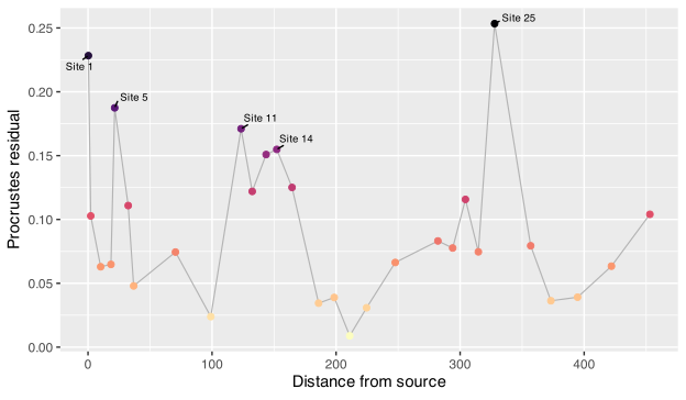
The environmental and fish ordinations are strongly concordant overall, but their local mismatches are especially informative. A symmetric Procrustes rotation superimposes the first two axes of the environmental PCA and the Bray-Curtis PCoA, while PROTEST asks whether that agreement is stronger than expected after permuting site identities.
```{r code-procrustes}
#| echo: false
env_proc_scores <- scores(
env_pca,
display = "sites",
choices = 1:2
)[keep, ]
fish_proc_scores <- scores(
spe_pcoa,
display = "sites",
choices = 1:2
)
set.seed(743)
proc_test <- protest(
env_proc_scores,
fish_proc_scores,
permutations = 999
)
proc_fit <- procrustes(
env_proc_scores,
fish_proc_scores,
symmetric = TRUE
)
proc_dat <- tibble(
site = as.integer(rownames(spe)),
dfs = site_dfs,
mismatch = residuals(proc_fit)
)
proc_top <- proc_dat |>
slice_max(mismatch, n = 5)
```
```{r fig-procrustes}
#| label: fig-procrustes
#| fig-cap: "Site-level mismatch after Procrustes rotation of the environmental PCA and fish-community PCoA. Large residuals mark sites whose fish composition departs most from the configuration expected from the first two environmental axes."
#| fig-width: 6.5
#| fig-height: 3.8
#| echo: false
ggplot(proc_dat, aes(dfs, mismatch)) +
geom_line(colour = "grey70", linewidth = 0.4) +
geom_point(aes(colour = mismatch), size = 1.8) +
geom_text_repel(
data = proc_top,
aes(label = paste("Site", site)),
size = 2.5,
min.segment.length = 0
) +
scale_colour_viridis_c(option = "magma", direction = -1, guide = "none") +
labs(
x = "Distance from source",
y = "Procrustes residual"
)
```
The two configurations have a Procrustes correlation of `r fmt(proc_test$t0, 3)` ($p = `r fmt(proc_test$signif, 3)`$), so environmental position and fish composition share a strong two-dimensional structure. The residual profile adds information that the global coefficient hides (@fig-procrustes). Site 25 is the largest mismatch and lies at the downstream edge of the oxygen-sag reach; sites 1 and 5 are also conspicuous at the species-poor headwater end. They are diagnostic sites where the dominant environmental axes leave more community structure unexplained, and therefore the first places to investigate omitted habitat, connectivity, disturbance, or sampling effects.
### Clustering the river into reaches
The preceding analyses describe the river as a long gradient interrupted by a short oxygen sag, so I can use a cluster analysis to turn that pattern into a partition of river segments. This is an indicative/exploratory grouping of sites under the same position and oxygen-stress variables that explained the fish composition.
```{r code-cluster}
reach_vars <- c("dfs", "oxy", "bod")
reach_hc <- hclust(dist(E[, reach_vars]), method = "complete")
reach_raw <- cutree(reach_hc, k = 3)

reach_lookup <- tibble(
  raw = reach_raw,
  dfs = site_dfs,
  bod = env_matched$bod
) |>
  summarise(
    mean_dfs = mean(dfs),
    mean_bod = mean(bod),
    .by = raw
  )

impacted_raw <- reach_lookup$raw[which.max(reach_lookup$mean_bod)]
mouth_raw <- reach_lookup |>
  filter(raw != impacted_raw) |>
  slice_max(mean_dfs, n = 1) |>
  pull(raw)
upper_raw <- setdiff(reach_lookup$raw, c(impacted_raw, mouth_raw))

reach_labels <- setNames(
  c(
    "Upper and pre-impact stretch",
    "Impacted oxygen-sag stretch",
    "Mouthward recovery stretch"
  ),
  c(upper_raw, impacted_raw, mouth_raw)
)

reach_dat <- tibble(
  site = as.integer(rownames(spe)),
  dfs = site_dfs,
  oxy = env_matched$oxy,
  bod = env_matched$bod,
  richness = rowSums(spe > 0),
  Reach = factor(
    reach_labels[as.character(reach_raw)],
    levels = c(
      "Upper and pre-impact stretch",
      "Impacted oxygen-sag stretch",
      "Mouthward recovery stretch"
    )
  )
)

reach_colours <- c(
  "Upper and pre-impact stretch" = "#2c7fb8",
  "Impacted oxygen-sag stretch" = "#b2182b",
  "Mouthward recovery stretch" = "#238b45"
)

site_span <- function(x) {
  full <- seq(min(x), max(x))
  missing <- setdiff(full, x)
  span <- paste0(min(x), "-", max(x))
  if (length(missing) == 0) {
    span
  } else {
    paste0(span, " (site ", paste(missing, collapse = ", "), " omitted)")
  }
}

reach_tab <- reach_dat |>
  summarise(
    Sites = site_span(site),
    n = n(),
    dfs_min = min(dfs),
    dfs_max = max(dfs),
    median_oxy = median(oxy),
    max_bod = max(bod),
    median_richness = median(richness),
    .by = Reach
  )
```
```{r fig-cluster-dendrogram}
#| label: fig-cluster-dendrogram
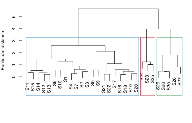
#| fig-cap: "Dendrogram from complete-linkage clustering of standardised distance from source, oxygen, and BOD. Rectangles mark the three-cluster solution used to define the reach groups."
#| fig-width: 7
#| fig-height: 4.5
old_par <- par(mar = c(5, 4, 1, 1))
plot(
  reach_hc,
  labels = paste0("S", reach_dat$site),
  xlab = "",
  sub = "",
  ylab = "Euclidean distance",
  main = ""
)
rect.hclust(
  reach_hc,
  k = 3,
  border = c("#2c7fb8", "#b2182b", "#238b45")
)
par(old_par)
```
```{r tbl-cluster}
#| label: tbl-cluster
#| tbl-cap: "Three reach clusters from complete-linkage hierarchical clustering of standardised distance from source, oxygen, and BOD."
reach_tab |>
  gt_doubs(
    note = "Clustering used `hclust(dist(scale(dfs, oxy, bod)), method = \"complete\")`; site 8 was omitted because it has no fish."
  ) |>
  cols_label(
    n = "n",
    dfs_min = "dfs min",
    dfs_max = "dfs max",
    median_oxy = "median oxygen",
    max_bod = "max BOD",
    median_richness = "median richness"
  ) |>
  fmt_number(
    columns = c(dfs_min, dfs_max, median_oxy, max_bod, median_richness),
    decimals = 1
  ) |>
  tab_style(
    style = cell_fill(color = "#fde0dd"),
    locations = cells_body(
      rows = Reach == "Impacted oxygen-sag stretch"
    )
  )
```
```{r fig-cluster}
#| label: fig-cluster
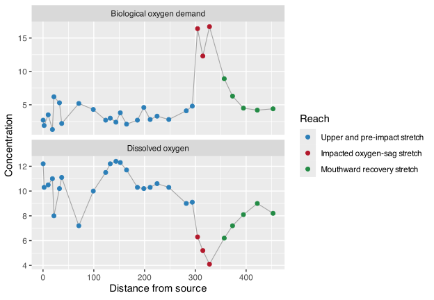
#| fig-cap: "Reach clusters along the river, shown against oxygen and BOD. The cluster analysis separates a broad upstream pre-impact stretch, the oxygen-sag reach, and the mouthward recovery stretch."
#| fig-width: 6.5
#| fig-height: 4.5
#| code-fold: true
reach_env_long <- reach_dat |>
  dplyr::select(dfs, Reach, oxy, bod) |>
  pivot_longer(
    cols = c(oxy, bod),
    names_to = "Variable",
    values_to = "value"
  ) |>
  mutate(
    Variable = recode(
      Variable,
      oxy = "Dissolved oxygen",
      bod = "Biological oxygen demand"
    )
  )

ggplot(reach_env_long, aes(dfs, value)) +
  geom_line(aes(group = Variable), colour = "grey65", linewidth = 0.4) +
  geom_point(aes(colour = Reach), size = 1.8) +
  facet_wrap(~Variable, ncol = 1, scales = "free_y") +
  scale_colour_manual(values = reach_colours) +
  labs(
    x = "Distance from source",
    y = "Concentration",
    colour = "Reach"
  )
```
The three-cluster solution gives a clean, interpretable partition (@fig-cluster-dendrogram; @tbl-cluster). Sites 1 to 22 form an upper and pre-impact stretch. Sites 23 to 25 are separated as the impacted oxygen-sag stretch, where oxygen is lowest and BOD is highest. Sites 26 to 30 form the mouthward recovery stretch. In other words, clustering can recover the same three-part field interpretation: the river does not change only as a smooth continuum, because a short polluted reach interrupts the downstream sequence before the assemblage recovers toward the river mouth (@fig-cluster).
### Do the reaches support distinct fish assemblages?
```{r code-reach-inference}
#| echo: false
reach_bray <- vegdist(spe, method = "bray")
set.seed(743)
reach_adonis <- adonis2(
reach_bray ~ Reach,
data = reach_dat,
permutations = 999
)
reach_beta <- betadisper(reach_bray, reach_dat$Reach)
set.seed(743)
reach_dispersion <- permutest(reach_beta, permutations = 999)
reach_mv <- mvabund::mvabund(as.matrix(spe))
reach_fit <- mvabund::manyglm(
reach_mv ~ Reach,
data = reach_dat,
family = "negative.binomial"
)
set.seed(743)
reach_anova <- anova(
reach_fit,
p.uni = "adjusted",
nBoot = 999,
test = "LR",
show.time = "none"
)
reach_tests <- tibble(
Code = colnames(spe),
deviance = reach_anova$uni.test[2, ],
adjusted_p = reach_anova$uni.p[2, ]
)
reach_means <- as_tibble(spe) |>
mutate(Reach = reach_dat$Reach) |>
summarise(across(where(is.numeric), mean), .by = Reach) |>
mutate(
Reach = recode(
as.character(Reach),
"Upper and pre-impact stretch" = "Upper",
"Impacted oxygen-sag stretch" = "Oxygen sag",
"Mouthward recovery stretch" = "Recovery"
)
) |>
pivot_longer(-Reach, names_to = "Code", values_to = "mean_abundance") |>
pivot_wider(names_from = Reach, values_from = mean_abundance)
reach_species <- reach_tests |>
filter(adjusted_p <= 0.05) |>
arrange(desc(deviance)) |>
slice_head(n = 8) |>
mutate(Species = unname(species_names[Code]), .after = Code) |>
left_join(reach_means, by = "Code")
```
The river segment groups were defined from distance, oxygen, and BOD rather than from the fish table, so the fish provide a separate biological check. The Bray-Curtis PERMANOVA attributes `r fmt(100 * reach_adonis$R2[1], 1)`% of compositional variation to reach ($p = `r fmt(reach_adonis[["Pr(>F)"]][1], 3)`$). Dispersion also differs among reaches ($p = `r fmt(reach_dispersion$tab[1, "Pr(>F)"], 3)`$), however, so the PERMANOVA cannot be read as a pure shift in group centroids. The oxygen-sag group is both compositionally displaced and unusually species-poor.
```{r tbl-reach-species}
#| label: tbl-reach-species
#| tbl-cap: "Species contributing most strongly to fish-assemblage differences among the three environmentally defined reaches."
#| echo: false
reach_species |>
dplyr::select(
Code,
Species,
Upper,
`Oxygen sag`,
Recovery,
adjusted_p
) |>
gt_doubs(
note = "Mean observed abundance by reach; adjusted resampling p-values from a negative-binomial manyGLM. The table shows the eight largest species-level deviances among taxa with adjusted p <= 0.05."
) |>
cols_label(adjusted_p = "adjusted p") |>
fmt_number(columns = c(Upper, `Oxygen sag`, Recovery), decimals = 1) |>
fmt_number(columns = adjusted_p, decimals = 3) |>
data_color(
columns = c(Upper, `Oxygen sag`, Recovery),
palette = c("#f7fbff", "#2171b5")
)
```
The negative-binomial manyGLM confirms an overall river segment effect ($p = `r fmt(reach_anova$table[["Pr(>Dev)"]][2], 3)`$) without relying on Bray-Curtis dispersion. The species results sharpen the interpretation (@tbl-reach-species): minnow, stone loach, and brown trout characterise the upper assemblage, whereas eel, ide, pumpkinseed, crucian carp, and ruffe rise in the recovery reach. None of the strongest differentiating taxa peaks in the oxygen-sag segment. Its identity is therefore defined mainly by assemblage depletion, not by a new set of specialist fishes, which anticipates the nestedness result in the next section.
### Replacement or loss? Beta-diversity partitioning
I have repeatedly called the downstream change a *replacement* of species. Beta-diversity partitioning tests that word by separating balanced turnover from the abundance-gradient component, the nestedness-like part where one assemblage is a thinned version of another.
```{r code-betapart}
library(betapart)
bp <- beta.multi.abund(spe, index.family = "bray")

beta_tab <- tibble(
  Component = c(
    "Total (beta.BRAY)",
    "Balanced turnover (replacement)",
    "Abundance gradient (nestedness-like)"
  ),
  Value = c(bp$beta.BRAY, bp$beta.BRAY.BAL, bp$beta.BRAY.GRA),
  Share = c(1, bp$beta.BRAY.BAL / bp$beta.BRAY, bp$beta.BRAY.GRA / bp$beta.BRAY)
)
```
```{r tbl-betapart}
#| label: tbl-betapart
#| tbl-cap: "Multi-site beta-diversity of the fish assemblage, split into balanced turnover and abundance-gradient components (Baselga family, abundance-based)."
beta_tab |>
  gt_doubs(note = "`betapart::beta.multi.abund()`, Bray-Curtis family.") |>
  fmt_number(columns = c(Value, Share), decimals = 3) |>
  tab_style(
    style = cell_fill(color = "#eef6ff"),
    locations = cells_body(
      rows = Component == "Balanced turnover (replacement)"
    )
  )
```
Turnover dominates, at about 0.86 of the total against 0.14 for the abundance-gradient component (@tbl-betapart). So, the word *replacement* is justified. The abundance-gradient component is small but present, and it is largest where the assemblage thins to a subset of the fuller lowland fauna, namely at the species-poor headwater and at the polluted mid-river reach. Beta-diversity partitioning recovers both processes and shows which one dominates.
### Which sites and species are distinctive? LCBD and SCBD
Local contributions to beta diversity (LCBD) rank sites by how much each adds to the total community variation. A high-LCBD site is ecologically distinctive, and a permutation test shows whether its distinctiveness exceeds chance. This analysis identifies the pollution reach without any prior specification of where to look.
```{r code-lcbd}
set.seed(743)
bd <- adespatial::beta.div(spe, method = "hellinger", nperm = 999)

lcbd_tab <- tibble(
  Site = as.integer(rownames(spe)),
  dfs = env_matched$dfs,
  LCBD = as.numeric(bd$LCBD),
  p = as.numeric(bd$p.LCBD)
) |>
  arrange(desc(LCBD)) |>
  slice_head(n = 6)
```
```{r tbl-lcbd}
#| label: tbl-lcbd
#| tbl-cap: "The six sites contributing most to total beta diversity, with distance from source and the permutation p-value."
lcbd_tab |>
  gt_doubs(note = "`adespatial::beta.div()`, Hellinger, 999 permutations.") |>
  fmt_number(columns = dfs, decimals = 1) |>
  fmt_number(columns = LCBD, decimals = 4) |>
  fmt_number(columns = p, decimals = 3) |>
  tab_style(
    style = cell_text(color = "#b2182b", weight = "bold"),
    locations = cells_body(columns = p, rows = p <= 0.05)
  )
```
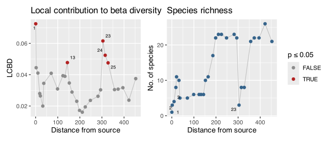
The most distinctive sites are the extreme headwater, a near-monospecific brown-trout reach, and sites 23 to 25 (@tbl-lcbd). @fig-lcbd shows every site's LCBD and species richness along the river. Richness collapses from 22 species to 3 at the pollution reach, exactly where LCBD peaks, before the assemblage recovers downstream.
```{r fig-lcbd}
#| label: fig-lcbd
#| fig-cap: "Local contribution to beta diversity (left) and species richness (right) along distance from source. Firebrick points mark sites significant at p ≤ 0.05."
#| fig-width: 7
#| fig-height: 3
#| code-fold: true
lcbd_plot <- tibble(
  site = as.integer(rownames(spe)),
  dfs = env_matched$dfs,
  LCBD = as.numeric(bd$LCBD),
  p = as.numeric(bd$p.LCBD),
  richness = rowSums(spe > 0)
) |>
  mutate(signif = p <= 0.05)

p1 <- ggplot(lcbd_plot, aes(dfs, LCBD)) +
  geom_line(colour = "grey75", linewidth = 0.4) +
  geom_point(aes(colour = signif), size = 1.8) +
  geom_text_repel(
    data = filter(lcbd_plot, signif),
    aes(label = site),
    size = 2.4
  ) +
  scale_colour_manual(
    values = c("FALSE" = "grey55", "TRUE" = "firebrick"),
    name = "p ≤ 0.05"
  ) +
  labs(
    title = "Local contribution to beta diversity",
    x = "Distance from source"
  )

p2 <- ggplot(lcbd_plot, aes(dfs, richness)) +
  geom_line(colour = "grey75", linewidth = 0.4) +
  geom_point(colour = "steelblue4", size = 1.8) +
  geom_text_repel(
    data = filter(lcbd_plot, richness <= 4),
    aes(label = site),
    size = 2.4
  ) +
  labs(
    title = "Species richness",
    x = "Distance from source",
    y = "No. of species"
  )

p1 + p2 + plot_layout(guides = "collect")
```
### A model-based check with manyGLM
Every distance-based method treats the count table through a dissimilarity index. `manyGLM()` instead fits a negative-binomial GLM to each species and tests the predictors jointly by resampling. It is a useful check that the ordination result does not depend on the Bray-Curtis geometry.
```{r code-manyglm}
library(mvabund)
Y <- mvabund(as.matrix(spe))
mg_fit <- manyglm(Y ~ dfs + bod + oxy, data = E, family = "negative.binomial")
set.seed(743)
mg_anova <- anova(mg_fit, p.uni = "none", nBoot = 199, test = "LR")
mg_anova$table
```
Distance from source, BOD, and oxygen are each significant, and distance from source has much the largest deviance. A method that makes the count distribution explicit reaches the same ranking as the ordinations.
### The shape of species responses
The ordinations assume, through the $\chi^2$ and Bray-Curtis geometries, that species rise and fall along the gradient rather than climb without limit. Species-level response models check that assumption directly. A significant negative quadratic term is a unimodal response with an optimum inside the surveyed reach, and the optimum is the fitted peak.
```{r code-response}
library(MASS)
focus <- c("Satr", "Cogo", "Thth", "Babl", "Baba", "Gogo", "Ruru", "Abbr")
sp_names <- species_names[focus]
dfs <- env_matched$dfs

response_tab <- map_dfr(focus, function(s) {
  fit <- glm.nb(spe[[s]] ~ dfs + I(dfs^2))
  co <- coef(fit)
  p2 <- summary(fit)$coefficients["I(dfs^2)", "Pr(>|z|)"]
  peak <- if (co[["I(dfs^2)"]] < 0) {
    -co[["dfs"]] / (2 * co[["I(dfs^2)"]])
  } else {
    NA_real_
  }
  in_range <- !is.na(peak) && peak >= min(dfs) && peak <= max(dfs)
  tibble(
    Code = s,
    Species = sp_names[s],
    Optimum = if (in_range) round(peak) else NA_real_,
    quad_p = p2,
    Response = if (in_range && p2 < 0.05) {
      "Unimodal, optimum in survey"
    } else {
      "Increasing, optimum below survey"
    }
  )
})
```
```{r tbl-response}
#| label: tbl-response
#| tbl-cap: "Negative-binomial response models against distance from source, with the fitted optimum and the quadratic-term p-value for each species."
response_tab |>
  gt_doubs(
    note = "`MASS::glm.nb(y ~ dfs + I(dfs^2))`; optimum in km from source."
  ) |>
  cols_label(quad_p = "quadratic p", Optimum = "optimum (km)") |>
  fmt_number(columns = quad_p, decimals = 3) |>
  sub_missing(columns = Optimum, missing_text = "beyond survey") |>
  tab_style(
    style = cell_fill(color = "#eef6ff"),
    locations = cells_body(rows = str_detect(Response, "Unimodal"))
  )
```
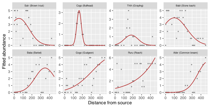
The pattern in @tbl-response and @fig-response is the ecology of the river in one picture. The headwater and mid-river species have clear optima ordered along the channel, from brown trout near 50 km to barbel near 350 km. The lowland species, roach, gudgeon, and common bream, are still climbing at the downstream limit, so their fitted optima lie beyond the sampled reach. This is the expected signature of a gradient sampled from its cold, species-poor source to a lower reach that has not yet reached the true lowland optima, and it is the same truncation that gives the DCA its long first axis.
```{r fig-response}
#| label: fig-response
#| fig-cap: "Fitted negative-binomial abundance responses (firebrick) with observed counts (grey) against distance from source. Vertical scales differ between panels."
#| fig-width: 7
#| fig-height: 3.6
#| code-fold: true
grid <- seq(min(dfs), max(dfs), length.out = 200)
pred <- map_dfr(focus, function(s) {
  fit <- glm.nb(spe[[s]] ~ dfs + I(dfs^2))
  tibble(
    code = s,
    dfs = grid,
    fit = as.numeric(predict(fit, tibble(dfs = grid), type = "response"))
  )
})
obs <- map_dfr(focus, ~ tibble(code = .x, dfs = dfs, abundance = spe[[.x]]))
lab <- setNames(paste0(focus, " (", sp_names[focus], ")"), focus)
pred$label <- factor(lab[pred$code], levels = lab[focus])
obs$label <- factor(lab[obs$code], levels = lab[focus])

ggplot(pred, aes(dfs, fit)) +
  geom_point(data = obs, aes(dfs, abundance), colour = "grey55", size = 0.7) +
  geom_line(colour = "firebrick", linewidth = 0.6) +
  facet_wrap(~label, scales = "free_y", ncol = 4) +
  labs(x = "Distance from source", y = "Fitted abundance") +
  theme(strip.text = element_text(size = 6))
```
::: {.callout-note appearance="simple"}
## What additional data would allow
The present data are a strong spatial snapshot, but some attractive advanced methods would answer questions the sampling design cannot support on its own.
* **Fish traits would permit RLQ and fourth-corner analysis.** These would test whether temperature, flow, oxygen, and substrate filter body size, trophic guild, reproductive strategy, or habitat preference rather than only changing species identities.
* **Repeated seasonal or annual surveys would permit joint species distribution models and multivariate trajectories.** They could separate persistent reach differences from year-to-year variation, estimate residual species associations, and test whether the oxygen-sag assemblage is stable or episodic.
* **True river-network coordinates and along-channel distances would permit directional stream-network models.** The present planar coordinates cannot represent flow-connected versus flow-unconnected sites, tributary junctions, or asymmetric downstream dispersal.
* **Reference reaches and before-after sampling would permit stronger impact inference.** A BACI design or an intervention-focused change-point model could distinguish the effect of an organic discharge from the natural downstream continuum more convincingly than this single-river correlation can.
:::
## A Decision Framework for Multivariate Analysis
After 24 chapters, the important question is no longer *which function do I run?* but *which ecological question am I asking?* @fig-decision-framework summarises the usual route. Start with the biological object, decide whether the aim is description, explanation, grouping, uniqueness, or species-level response, and then choose the method whose assumptions match that aim.
```{mermaid}
%%| label: fig-decision-framework
%%| fig-cap: "A practical decision framework for choosing among the multivariate methods used in the module."
%%{init: {"flowchart": {"wrappingWidth": 420}}}%%
flowchart TB
  A["Start with the ecological question"] --> B

  B["1. What is the response table?<br/><br/>Environmental variables → PCA<br/>Species community → continue downward"]
  B -->|"For a community table"| C

  C["2. Describe composition without predictors?<br/><br/>Short or linear gradient → Hellinger PCA or RDA<br/>Long or unimodal gradient → CA or DCA<br/>Dissimilarity-based analysis → PCoA or nMDS"]
  C -->|"If explanation is required"| D

  D["3. Explain composition with predictors?<br/><br/>Linear responses → RDA · Unimodal responses → CCA<br/>Dissimilarity-based response → db-RDA<br/>Environment and space overlap → variation partitioning and MEM"]
  D -->|"For another analytical aim"| E

  E["4. Compare or classify sites?<br/><br/>Compare configurations → Procrustes and PROTEST<br/>Test predefined groups → PERMANOVA plus dispersion<br/>Create groups → cluster analysis"]
  E -->|"To locate ecological contributions"| F

  F["5. Which sites or species make the pattern?<br/><br/>Distinctive sites or species → LCBD and SCBD<br/>Replacement versus abundance loss → beta-diversity partitioning<br/>Species-level inference → manyGLM or response GLMs"]

  classDef start fill:#243447,color:#ffffff,stroke:#243447,stroke-width:2px;
  classDef question fill:#eef6ff,color:#182536,stroke:#4f6f8f,stroke-width:1.5px;
  classDef final fill:#f4f8f3,color:#182536,stroke:#568060,stroke-width:1.5px;
  class A start;
  class B,C,D,E question;
  class F final;
```
The framework is deliberately not a recipe. Several methods may be defensible for the same dataset, as the Doubs example shows. The strongest analysis is usually the one in which several defensible methods answer neighbouring questions and converge on the same ecological interpretation.
## Synthesis: One Continuum and One Interruption
These analyses show that the Doubs assemblage is organised primarily by a longitudinal river continuum. The upper sites are high, steep, cool reaches with near-saturated oxygen and little nutrient load, while the lower sites are further from source, warmer, harder, and more enriched. Every unconstrained method recovered the same upstream-to-downstream gradient. Every constrained method selected variables describing river position and oxygen conditions. Every spatial analysis showed that environmental and geographic structure coincide along a river channel. Procrustes analysis then showed that the environmental and fish configurations are strongly aligned overall while exposing a small set of local mismatches. The model-based analyses confirmed that the broad pattern is a replacement of trout-zone species by lowland fishes, not only a change in a multivariate score.
The continuum is not perfectly smooth, and the most valuable results show where the gradient is interrupted. A short river stretch at sites 23 to 25 has a strong organic-load signal with oxygen falling to 4 mg L^-1^ and BOD above 12, and the fauna there thins to a few tolerant species before recovering. That stretch is the reason oxygen and BOD survive forward selection where nitrate does not. It has the highest LCBD outside the headwater, it supplies most of the nestedness-like component of beta diversity, it forms its own reach in the cluster analysis, and it is visible as the richness minimum in @fig-lcbd. The reach-level manyGLM adds an important detail: the impacted reach has no distinctive specialist fauna among the strongest species responses; it is defined by the disappearance of both upper-river and recovering lowland taxa. Overall, the analyses describe two overlaid gradients, a long physical-chemical continuum and a short, sharp oxygen sag, not the single monotonic trend the earlier chapters revealed.
The method families therefore fit together rather than compete. Ordination describes the dominant structure. Constrained ordination connects that structure to measured predictors. Spatial methods show why environment and geography cannot be cleanly separated in one river. Procrustes analysis tests whether two views of the sites agree and locates their exceptions. Clustering turns the interpretation into named reaches, while PERMANOVA, dispersion, and manyGLM test what those groups mean biologically. LCBD, beta-diversity partitioning, and species response models then move from the whole assemblage back to the sites and species that make the pattern biologically real.
These conclusions are based on correlational evidence, so association is not mechanism, which is why the [selection argument](#sec-selection) did not name a single driver. The gradient is truncated at both ends, so the optima of the most downstream species are situated beyond the survey. Environment and space are confounded along a single channel, which is why the shared fraction of the variation partition is so large. These are properties of one river surveyed once, and they would be relaxed only by more rivers, more seasons, or experimental work.
```{r code-session}
#| code-fold: true
sessioninfo::session_info(
  pkgs = c("vegan", "leaflet", "adespatial", "betapart", "mvabund", "gt")
)$packages |>
  as_tibble() |>
  filter(
    package %in%
      c(
        "vegan",
        "leaflet",
        "adespatial",
        "betapart",
        "mvabund",
        "gt",
        "MASS"
      )
  ) |>
  dplyr::select(package, loadedversion, source)
```