
- The history of climate-change science, from early experiments to sustained atmospheric measurements.
- Early estimates by Callendar and Plass compared with current global rates.
- The carbon cycle, atmospheric CO2 accumulation and seasonal exchange.
- Instrumental temperature records, palaeoclimate CO2 and future emissions scenarios.
- Ocean uptake, ecological feedbacks and the consequences for plant ecophysiology.
This lecture explains how measurements and physical reasoning established the role of atmospheric CO2 in climate change. We follow the scientists who developed that understanding, compare their estimates with current evidence, and use the carbon cycle to interpret the trends. The African historical narrative and long scrolling graphic are in Lecture 4.
By the end of this lecture, you will be able to:
- Explain the contributions of Fourier, Pouillet, Foote, Tyndall, Arrhenius, Callendar, Plass and Keeling to climate-change science.
- Compare historical estimates with modern measurements while distinguishing warming rates, temperature anomalies and climate sensitivity.
- Trace carbon among the atmosphere, plants, soils, oceans and geological stores, distinguishing stocks from fluxes.
- Explain the seasonal CO2 cycle and why it can coexist with long-term atmospheric accumulation.
- Read current CO2 and temperature records, stating their spatial coverage, reference periods and uncertainty.
- Relate ocean uptake, feedbacks and future emissions scenarios to plant function and environmental stress.
- Callendar, G. S. (1938). The artificial production of carbon dioxide and its influence on temperature. Quarterly Journal of the Royal Meteorological Society, 64(275), 223–240.
- Plass, G. N. (1956). The carbon dioxide theory of climatic change. Tellus, 8(2), 140–154.
- Forster, P. M., and others (2026). Indicators of Global Climate Change 2025: annual update of key indicators of the state of the climate system and human influence. Earth System Science Data, 18(6), 3889–3933. (optional)
1 Introduction to the carbon cycle
Photosynthesis connects light, inorganic carbon and water with the production of organic matter. Respiration and decomposition return much of that carbon to the environment. Some remains in biomass, soils, ocean waters or sediments for longer periods. The amount in each store depends on the balance of transfers into and out of it.
Industrial activity changes this balance by transferring carbon from geological stores into the atmosphere. Land-use change also alters carbon storage and exchange. Climate change is one consequence within the wider set of global changes introduced in Lecture 1.
2 Historical development of climate change science
2.1 Fourier and Pouillet
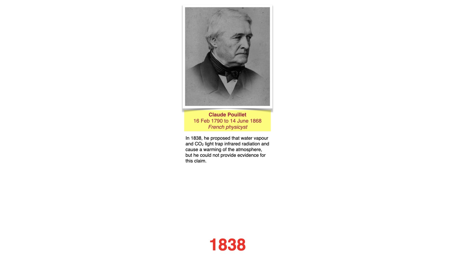
In the 1820s, Joseph Fourier considered Earth’s temperature as a problem of incoming and outgoing energy and recognised the atmosphere’s importance. In 1838, Claude Pouillet developed estimates of solar heating and atmospheric absorption. Their work established questions that later laboratory measurements and radiation calculations could address. The American Institute of Physics history of the greenhouse effect traces this development.

2.2 Eunice Foote
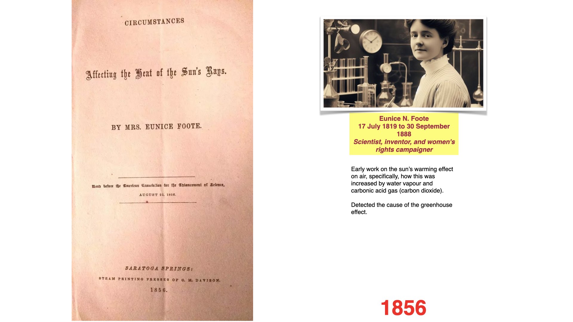
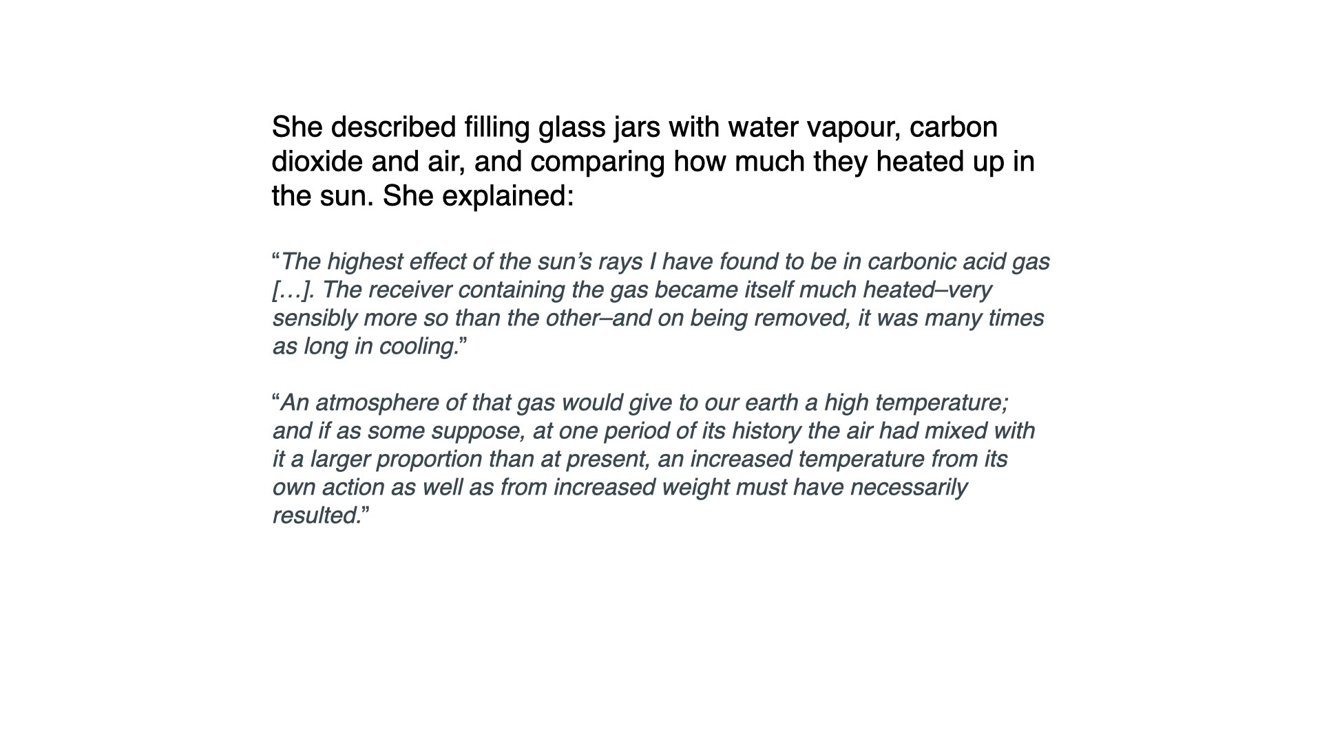
In 1856, Eunice Newton Foote compared the warming of gases in glass cylinders exposed to sunlight. The cylinder containing CO2 warmed strongly, and she inferred that an atmosphere richer in that gas could be warmer (Foote 1856). Her experiment and inference preceded Tyndall’s work. However, heating a sunlit cylinder involves several processes, so it should not be treated as an isolated measurement of the absorption of Earth’s outgoing infrared radiation. See the AIP comparison of Foote’s and Tyndall’s experiments.
2.3 John Tyndall
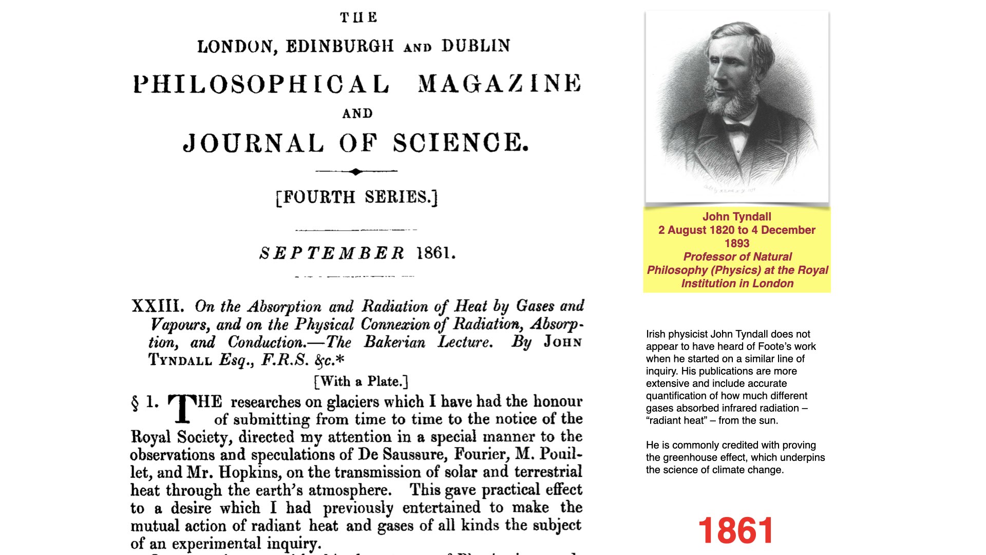
Tyndall’s experiments, first reported in 1859 and developed in his 1861 paper, measured the absorption of thermal radiation by gases. Water vapour and CO2 absorbed strongly in relevant infrared bands, whereas the main atmospheric gases, nitrogen and oxygen, absorbed much less (Tyndall 1861). This supplied a physical mechanism linking atmospheric composition with radiative energy exchange. His experiment differed from Foote’s sunlit cylinders in both apparatus and the radiation being investigated.
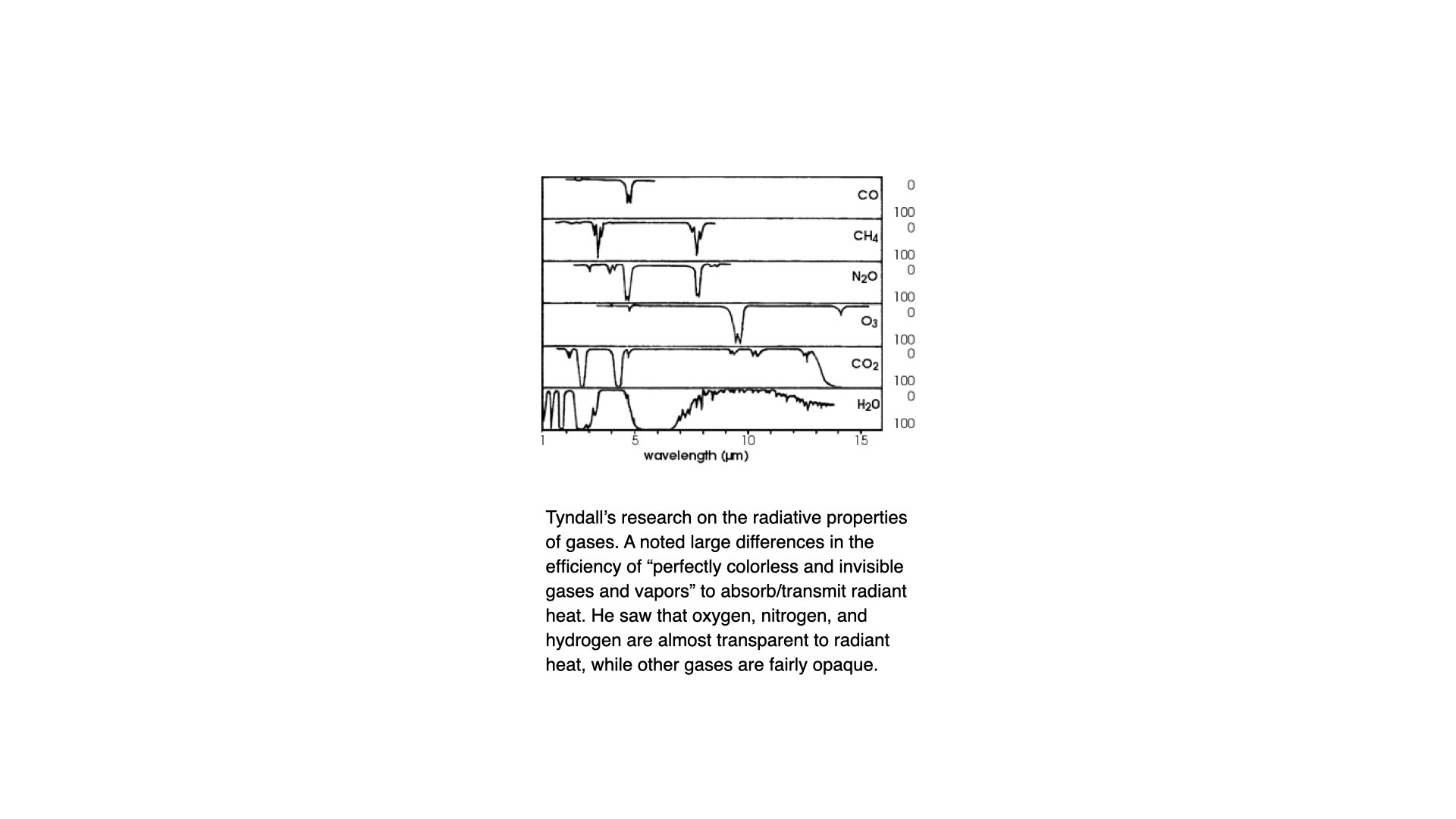
Today an infrared gas analyser, or IRGA, uses absorption in selected wavelength bands to estimate gas concentration after calibration. In a leaf chamber, the difference in CO2 between incoming and outgoing air can be used to estimate gas exchange. This connects the history of atmospheric physics with the plant measurements used in ecophysiology.
2.4 Svante Arrhenius
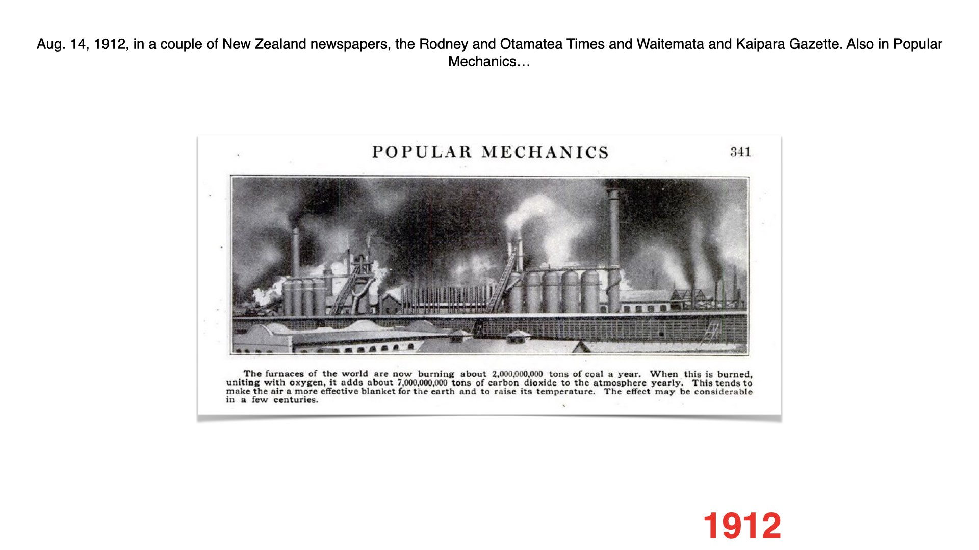
In 1896, Arrhenius used radiation calculations to estimate how changing atmospheric CO2 could affect surface temperature. His estimate for doubled CO2 was roughly 5–6 °C, with variation across his calculations (Arrhenius 1896). It was an early climate-sensitivity calculation, not a prediction of an annual warming rate. Modern calculations include better spectroscopy, ocean heat uptake and feedbacks. NASA’s account of early climate modelling explains the development.
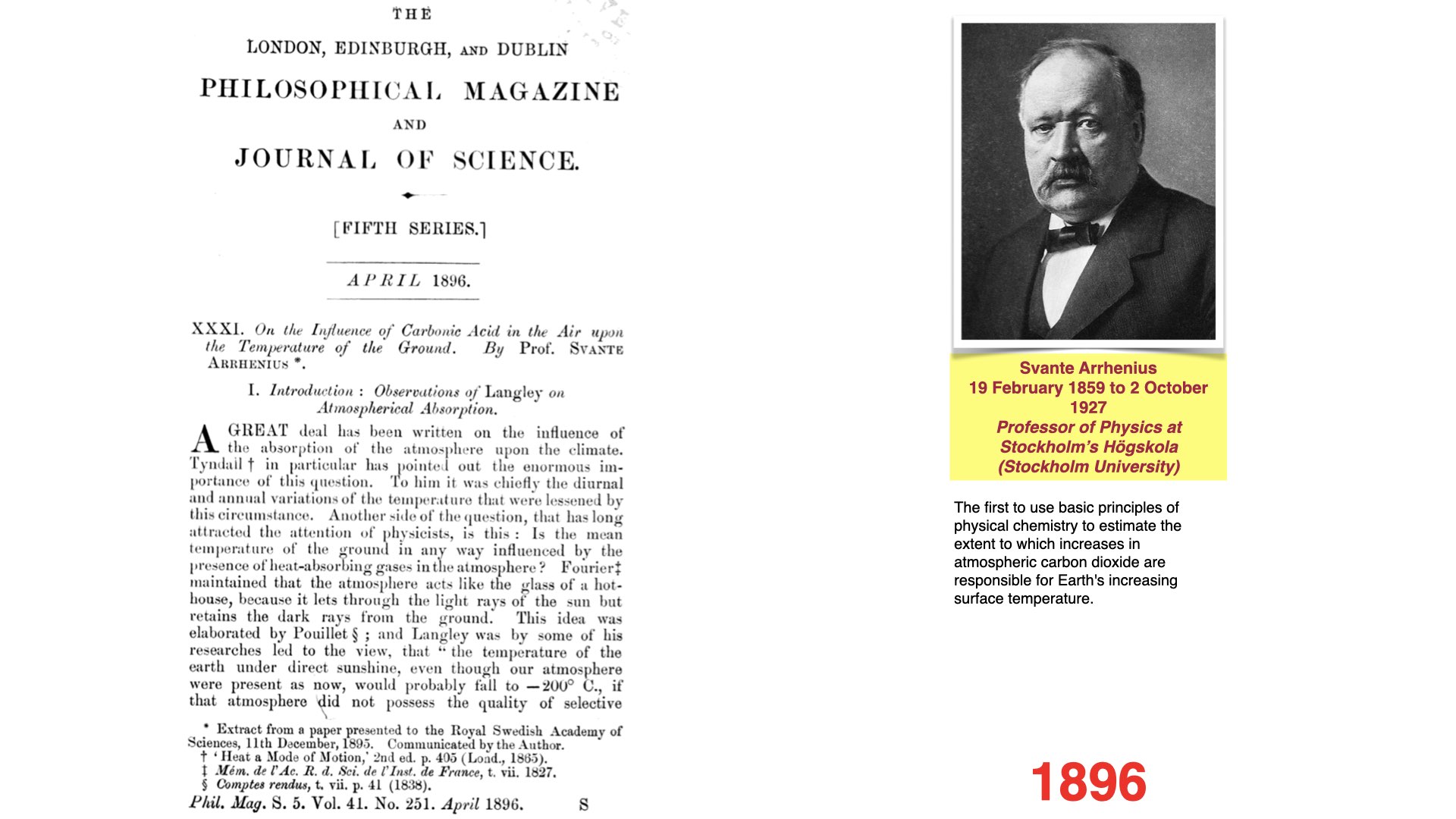
The coal-burning connection also reached the public. The 1912 newspaper item below is a historical example of that discussion, rather than the beginning of the scientific understanding.
2.5 Guy Stewart Callendar
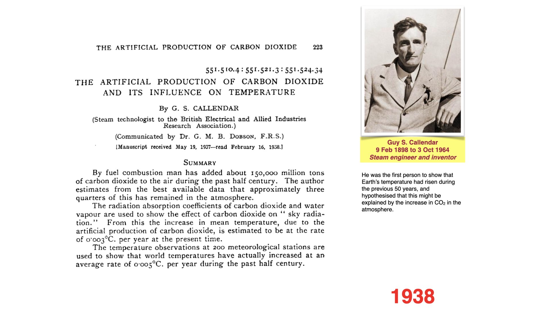
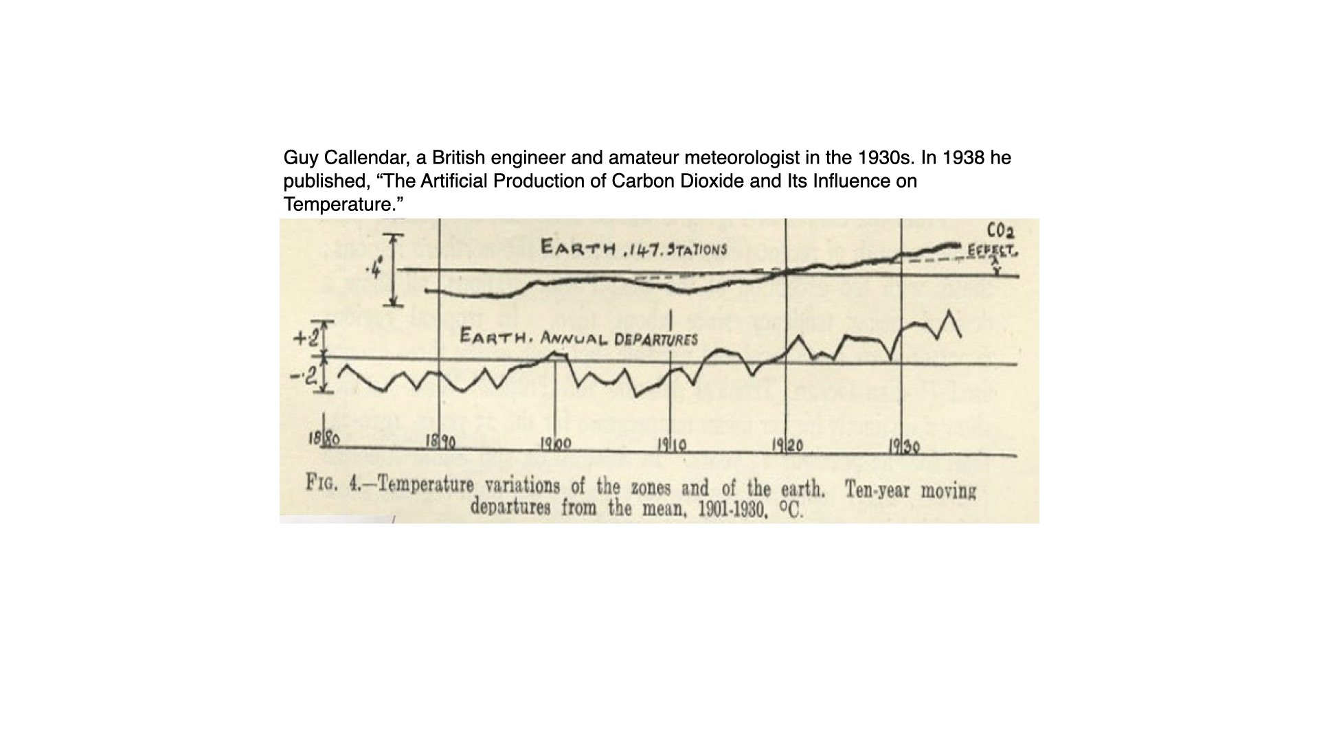
Callendar’s 1938 paper combined temperature observations with a calculation of the radiative effect of fossil-fuel CO2. He reported an observed warming rate of about 0.005 °C per year over the preceding half-century, and a separate estimated CO2-driven rate of 0.003 °C per year at the time. Distinguish the measured trend from the calculated contribution: they were different quantities even within the same paper (Callendar 1938).
2.6 Gilbert Plass
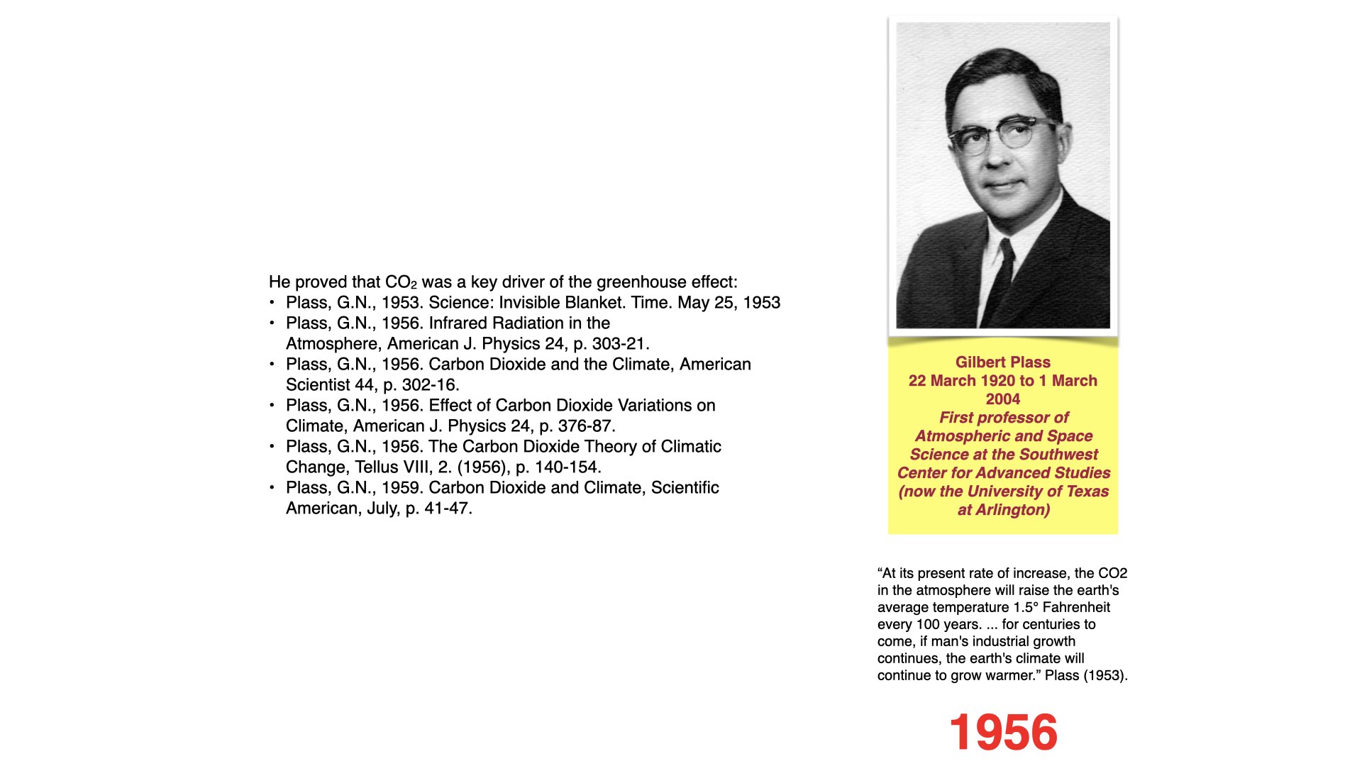
Plass used improved infrared calculations in the 1950s, including the effects of spectral lines and their overlap. In his 1956 paper he estimated 3.6 °C warming for doubled CO2 under his stated assumptions. He also estimated a CO2 increase of nearly 30% per century and warming of 1.1 °C per century under the industrial conditions he considered. Those rate estimates depend on their emissions and uptake assumptions (Plass 1956). The original paper is available here.
2.7 Charles David Keeling
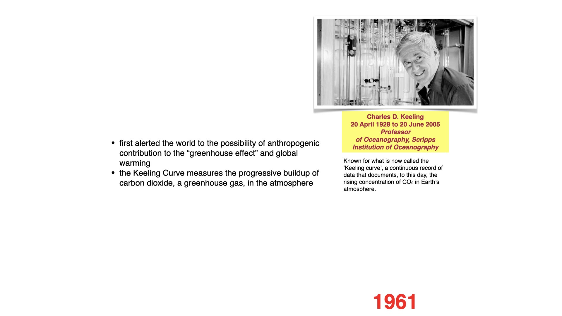
Keeling began sustained high-precision CO2 measurements at Mauna Loa in 1958. The resulting record resolved both an annual cycle and a persistent increase. It made changes in atmospheric composition directly observable over successive decades. Today the Mauna Loa series is complemented by a global network, so a measurement at one station can be compared with a spatially averaged record. See the Scripps history of the Keeling Curve.
3 Early estimates and current global rates
Read the units and averaging periods before comparing the numbers. A rate describes change per unit time. A temperature anomaly describes a difference from a reference mean. Climate sensitivity describes a response to a specified forcing. The modern values below are the latest complete-year or assessed-period values available in the 15 October 2026 data snapshot.
| Quantity and early source | Early estimate in common units | Current global comparison | How to interpret the comparison |
|---|---|---|---|
| Observed warming, Callendar (1938) | 0.005 °C yr⁻¹, or 0.05 °C per decade, over the preceding half-century | 0.0206 °C yr⁻¹, or 0.206 °C per decade: an ordinary least-squares trend through NASA GISTEMP annual means for 1976–2025 | Both cover roughly 50 years, but Callendar’s station coverage and the modern land–ocean index differ. |
| Calculated CO2-driven warming, Callendar (1938) | 0.003 °C yr⁻¹, or 0.03 °C per decade, under then-current conditions | Assessed human-induced warming: 0.027 °C yr⁻¹, or 0.27 [0.20–0.40] °C per decade, for 2016–2025 | The modern attribution includes human influences beyond CO2. It is not a direct measurement of the same simplified calculation. |
| Calculated warming, Plass (1956) | 0.011 °C yr⁻¹, or 0.11 °C per decade, converted from 1.1 °C per century | The same 0.27 [0.20–0.40] °C per decade assessed human-induced rate for 2016–2025 | Plass’s industrial and uptake assumptions differ from the subsequent emissions pathway. This is a historical comparison, not a forecast-skill test. |
| Atmospheric CO2 increase, Plass (1956) | Nearly 30% per century, equivalent to about 0.30% of his reference concentration per year on a linear basis | 2.06 ± 0.08 ppm yr⁻¹ in 2025; about 0.48% yr⁻¹ when divided by that year’s global mean, 425.62 ppm | The modern percentage is an explicitly normalised annual increment. Plass’s century-scale percentage is not a compound annual growth rate. |
For a separate comparison of CO2 doubling responses, Arrhenius’s roughly 5–6 °C, Callendar’s approximately 2 °C and Plass’s 3.6 °C can be set alongside the IPCC AR6 best estimate of equilibrium climate sensitivity of 3 °C, with a likely range of 2.5–4 °C. The historical calculations used different treatments of radiation and feedbacks. None of these doubling-response values is an annual warming rate (Arias et al. 2021).
4 Current atmospheric records
4.1 The Mauna Loa record
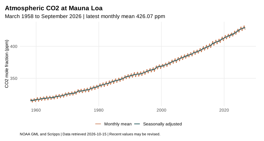
The upward movement and the annual oscillation answer different questions. The long-term increase records net accumulation in the atmosphere. The oscillation reflects seasonal exchange, especially with Northern Hemisphere vegetation. A fall over several months does not establish a fall from one complete year to the next.
NOAA’s series temporarily used observations from nearby Maunakea after the Mauna Loa eruption interrupted measurements in late November 2022; Mauna Loa measurements resumed in July 2023. This is documented in the source file.
4.2 A station record and a global mean
The global annual mean for 2025 was 425.62 ± 0.05 ppm, from NOAA’s marine boundary layer network. This differs from the Mauna Loa value because the station, spatial averaging and time interval differ. Use matched quantities when comparing sites or years. NOAA annual global means.
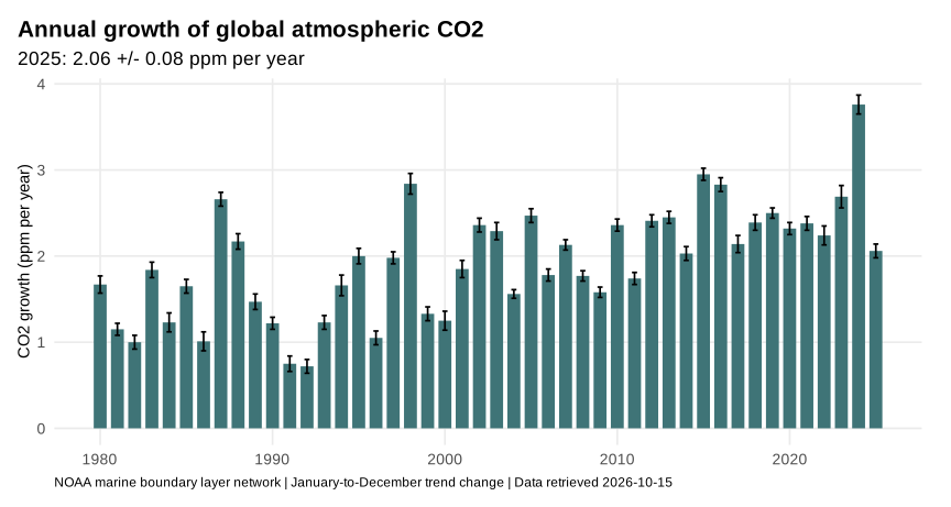
Concentration and growth rate are different quantities. NOAA’s 2025 growth rate is the change in the seasonally adjusted trend across that year. It is not simply the difference between the 2024 and 2025 annual means. A smaller positive growth rate still means that atmospheric CO2 is increasing. It also need not mean emissions have fallen: changes in land and ocean uptake affect the atmospheric balance.
4.3 Seasonal exchange and plant activity
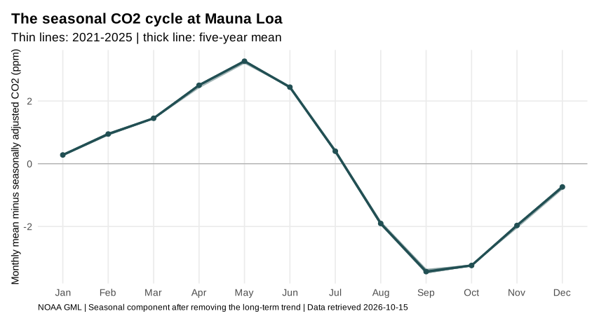
At Mauna Loa, CO2 usually reaches its seasonal maximum around May and its minimum around September or October. During the northern growing season, vegetation takes up carbon rapidly. Respiration and decomposition continue, but the seasonal balance shifts towards uptake. Later, reduced photosynthesis and continuing respiratory losses shift the balance towards atmospheric release. The phase and amplitude differ among stations, particularly between hemispheres. NOAA CO2 records.
The figure removes the long-term trend so that the within-year pattern can be examined directly. Its vertical axis is a seasonal departure in ppm, not the atmospheric concentration itself.
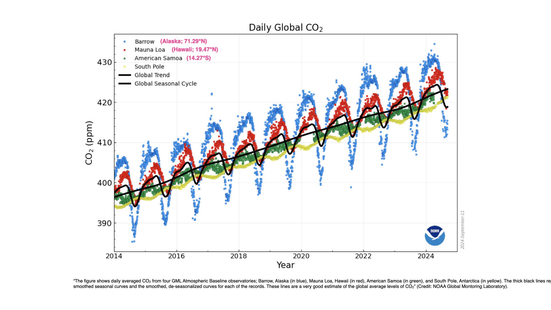
Both hemispheres show a sustained increase, but the northern stations show much larger seasonal excursions. Seasonal plant exchange, the distribution of land and vegetation, and atmospheric transport help explain these differences. Global mixing connects the records without making every station’s concentration identical.
Using Figure 2 and Figure 4, explain how seasonal plant activity can produce a recurring annual decline while the atmospheric concentration continues to rise over decades. State which months you are comparing and distinguish photosynthesis from net ecosystem carbon storage. This is a study exercise with no separate submission or continuous assessment mark. Assessed tasks and deadlines are in the module timetable.
5 Carbon stocks and fluxes
A stock is an amount of carbon in a defined store. A flux is a transfer per unit time. Atmospheric concentration is related to the atmospheric stock, whereas emissions, photosynthesis and ocean exchange are fluxes. The accounting can be written schematically as:
\[ \begin{aligned} \text{atmospheric carbon change per year} &= \text{fossil and land-use emissions}\\ &\quad - \text{net land uptake}\\ &\quad - \text{net ocean uptake}. \end{aligned} \]
Express every term in the same carbon units per year. Net uptake already subtracts the opposing release. Gross photosynthesis alone therefore cannot establish whether an ecosystem is a net carbon sink. Newly fixed carbon can be respired, decomposed, burned or exported. The system boundary and observation period matter, just as they do for nutrient budgets later in the module.
The ocean absorbs carbon through air–sea exchange, and circulation and biological processes redistribute it. Dissolved CO2 participates in carbonate chemistry, increasing hydrogen-ion concentration and lowering pH as more carbon is added. Ocean heat uptake also slows the rise in surface temperature while increasing ocean heat content. The WMO State of the Global Climate 2025 reports continuing ocean warming and acidification (World Meteorological Organization 2026).
A short reduction in emissions does not necessarily make atmospheric concentration decline: inputs can still exceed net uptake. Likewise, reaching net zero CO2 emissions is different from eliminating all environmental change. Sustained net zero CO2 is expected to approximately stabilise CO2-driven warming, while sea level and other slow components can continue changing (Lee et al. 2021).
6 CO₂ in palaeoclimate context
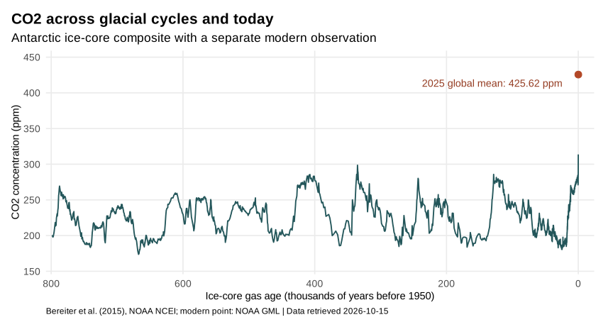
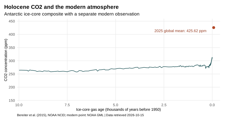
The ice-core curves use the revised composite assembled by Bereiter et al. (2015), archived by NOAA NCEI. They reconstruct past air from bubbles in Antarctic ice. The modern point is a direct atmospheric observation, not an additional ice-core sample. The time resolution and dating differ, so the two should not be treated as one uniformly sampled record.
CO2 changed naturally during glacial cycles. Its present concentration is nevertheless well above the late-Quaternary range represented here. For the African vegetation and human histories associated with those intervals, return to Lecture 4.
7 Current temperature records
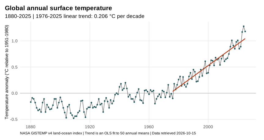
A temperature anomaly is a difference from a stated reference mean. NASA’s figure uses 1951–1980. The WMO multi-dataset assessment reports 2025 at 1.43 ± 0.13 °C above 1850–1900. These numbers use different baselines and methods, so their numerical values should not be compared as if they shared a zero. A single warm year also differs from the long-term warming level used in the Paris Agreement (World Meteorological Organization 2026).
The NASA 50-year trend in Table 1 is a descriptive fit to observations. The recent human-induced rate of 0.27 °C per decade is an attribution estimate over 2016–2025. It addresses a different period and separates human influence from natural drivers and internal variability. A fitted rate depends on the interval selected (Forster et al. 2026).
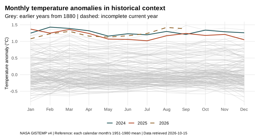
The figure shows monthly anomalies relative to each calendar month’s reference mean. The seasonal climate reference has already been subtracted month by month. Its month-to-month changes therefore describe departures from expected seasonal conditions. This differs from the CO2 seasonal cycle in Figure 4. NASA GISTEMP data.
8 Future emissions scenarios
Scenarios describe conditional futures under specified emissions and socioeconomic assumptions. They are not forecasts: each one asks what would follow if society developed in a particular way, and together they show the range of futures that depend on choices still to be made.
8.1 Representative concentration pathways
The IPCC Fifth Assessment Report (AR5) was built on four Representative Concentration Pathways (RCPs) (Vuuren et al. 2011). Each RCP is named after the radiative forcing it reaches in 2100, in watts per square metre: RCP2.6, RCP4.5, RCP6.0 and RCP8.5. Together they span the range of forcing in the published literature, from a pathway with strong mitigation (RCP2.6) to one with continued high emissions (RCP8.5). An RCP specifies greenhouse gas concentrations, emissions and land use over time; integrated assessment models then show what kind of energy system and economy could produce such a pathway.
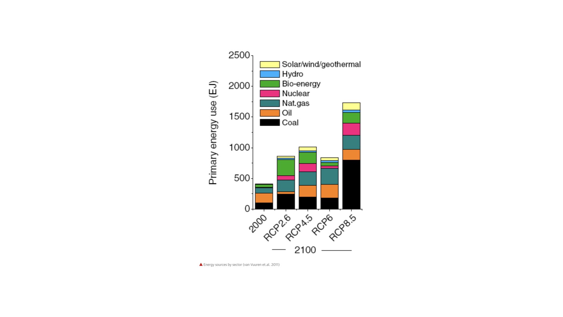
The energy systems behind the RCPs differ less in how much energy people use than in where it comes from. In all four pathways, global primary energy use in 2100 is about twice that of 2000 or more. In RCP8.5 it is roughly four times larger and is dominated by coal. In RCP2.6 the extra energy comes mostly from bio-energy, nuclear power and other low-carbon sources, with a much smaller share of coal and oil (Vuuren et al. 2011). Low and high emission futures are therefore distinguished mainly by the carbon content of the energy supply.
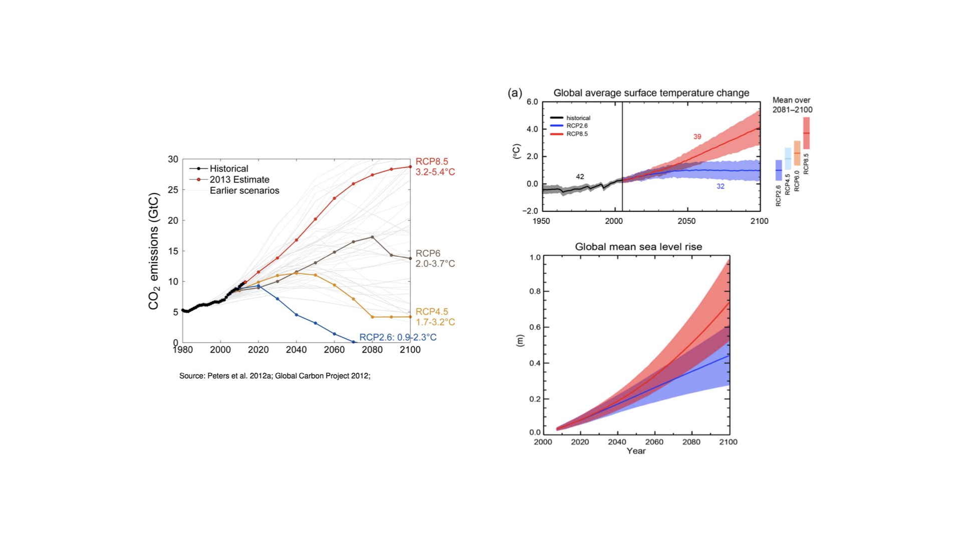
The left panel compares observed fossil CO2 emissions with the RCPs. By the early 2010s, emissions were following the upper end of the scenario range, close to RCP8.5, and the authors concluded that keeping warming below 2 °C would require immediate, large and sustained reductions in emissions (Peters et al. 2013). The warming ranges printed beside each pathway show how strongly the end-of-century outcome depends on the path taken, from about 0.9–2.3 °C for RCP2.6 to 3.2–5.4 °C for RCP8.5. The right panels show the AR5 projections for RCP2.6 and RCP8.5. For 2081–2100, relative to 1986–2005, the likely ranges of warming were 0.3–1.7 °C under RCP2.6 and 2.6–4.8 °C under RCP8.5, and of global mean sea-level rise 0.26–0.55 m and 0.45–0.82 m (IPCC 2013). The two pathways differ little until about the 2040s and separate in the second half of the century, because warming over the next few decades is set largely by emissions that have already occurred and by the slow response of the oceans.
9 Consequences for Plant Ecophysiology
Climate change alters the conditions under which plants acquire resources and maintain their tissues. Temperature affects metabolism and respiratory losses. Water availability and atmospheric drying demand affect stomatal opening and carbon gain. Marine plants also face changes in water temperature, carbonate chemistry, mixing and nutrient supply.
Rising CO2 can stimulate photosynthesis under some conditions, but water, nutrients, temperature and losses can restrict the resulting growth or storage. Drought, fire, mortality and decomposition can return carbon to the atmosphere. These responses connect plant physiology with the carbon cycle rather than providing an automatic increase in ecosystem carbon storage.
Mitigation changes the drivers, for example by reducing emissions or protecting carbon stores. Adaptation changes how people and ecosystems respond to the conditions they encounter. Keep these societal uses of the word adaptation distinct from inherited evolutionary adaptation and within-individual acclimatisation. Lecture 10 develops the physiological stress responses.
10 Summary
- Laboratory experiments and radiation calculations established the role of atmospheric CO2 in Earth’s energy balance long before sustained measurements began. Foote found that sunlit CO2 warmed strongly, and Tyndall measured the absorption of thermal radiation by CO2 and water vapour. Arrhenius, Callendar and Plass then estimated the warming that more CO2 would cause.
- Keeling’s Mauna Loa record, begun in 1958, made the rise in atmospheric CO2 directly observable. The global mean reached 425.62 ppm in 2025, and the 2025 growth rate was 2.06 ppm yr⁻¹.
- Warming rates, temperature anomalies and climate sensitivity are different quantities. Callendar’s observed 0.005 °C yr⁻¹ compares with a modern NASA trend of 0.206 °C per decade for 1976–2025, whereas the 5–6 °C, 3.6 °C and 3 °C values of Arrhenius, Plass and IPCC AR6 are responses to doubled CO2.
- A stock is an amount of carbon in a store and a flux is a transfer per unit time. Atmospheric CO2 rises whenever fossil and land-use emissions exceed net uptake by land and ocean.
- The seasonal CO2 cycle, largest at Northern Hemisphere stations, reflects the balance between photosynthesis and respiration through the year, and it is superimposed on a long-term increase.
- Antarctic ice cores show CO2 mostly between about 180 and 300 ppm over the last 800,000 years, well below the present concentration.
- Scenarios (the RCPs of AR5 and the SSPs of AR6) are conditional futures, not forecasts; low and high emission pathways differ mainly in the carbon content of the energy supply.
- Future warming depends on the emissions pathway, from 1.8 °C under SSP1-2.6 to 4.4 °C under SSP5-8.5 for 2081–2100 relative to 1850–1900.
- Rising CO2, temperature and drought alter photosynthesis, respiration and water use, but they do not automatically increase ecosystem carbon storage.
11 Self-test questions
Foote (1856) showed that a sunlit glass cylinder containing CO2 warmed strongly, and inferred that an atmosphere with more CO2 could be warmer. Tyndall (1859, 1861) measured the absorption of thermal radiation by gases, showing that water vapour and CO2 absorb strongly in infrared bands while nitrogen and oxygen absorb much less. Keeling began sustained high-precision CO2 measurements at Mauna Loa in 1958, which recorded both the annual cycle and the long-term increase. Foote’s sunlit cylinders involved several heating processes, whereas Tyndall isolated the absorption of thermal radiation by each gas.
0.005 °C yr⁻¹ × 10 = 0.05 °C per decade. The modern trend is 0.206 °C per decade, so 0.206 / 0.05 ≈ 4.1 times faster. Both rates cover roughly 50 years, but Callendar used land stations available in the 1930s, whereas GISTEMP is a global land–ocean index with different coverage and methods.
- Climate sensitivity: Plass’s estimated warming for doubled CO2, comparable with the IPCC AR6 best estimate of 3 °C. (b) A warming rate: the assessed human-induced warming per decade over a stated period. (c) A temperature anomaly: the 2025 temperature as a difference from the 1850–1900 reference mean. Only values of the same kind, with the same reference period, can be compared directly.
During the northern growing season, photosynthesis by Northern Hemisphere vegetation takes up carbon faster than respiration and decomposition release it, so atmospheric CO2 falls. Later in the year, photosynthesis declines while respiration continues, and CO2 rises again. Over a whole year, fossil and land-use emissions exceed net uptake by land and ocean, so the seasonally adjusted concentration keeps rising. Barrow is in the Northern Hemisphere, which has most of the land and seasonal vegetation, whereas the South Pole is far from large areas of seasonal plant growth.
2.06 / 425.62 × 100 ≈ 0.48% yr⁻¹. The growth rate was positive, so atmospheric CO2 still increased in 2025, only more slowly than in 2024. The growth rate is the balance of emissions and net land and ocean uptake, so a smaller increase can come from greater uptake in that year without any fall in emissions.
Water, nutrients and temperature can limit the growth that extra photosynthesis would otherwise support. Newly fixed carbon can be respired, decomposed, burned or exported, so gross photosynthesis does not establish net storage. Drought, fire and mortality can also return stored carbon to the atmosphere.
Warming over the next few decades is set largely by emissions that have already occurred and by the slow response of the oceans, so the pathways separate only later in the century. RCP8.5 assumes continued high emissions from an energy system that, by 2100, uses about four times the primary energy of 2000 and relies heavily on coal; RCP2.6 assumes a supply dominated by bio-energy, nuclear and other low-carbon sources.
12 Figure data and sources
The current figures use data retrieved on 15 October 2026. The monthly observational records extend through September 2026; complete annual comparisons end in 2025. Recent observations remain subject to their providers’ quality control and revision.
- NOAA and Scripps Mauna Loa monthly CO2.
- NOAA global annual CO2 means and global growth rates.
- NASA GISTEMP v4, with the land–ocean temperature table.
- Bereiter et al. (2015), revised Antarctic ice-core CO2 composite.
- Forster et al. (2026), Indicators of Global Climate Change 2025.
- WMO State of the Global Climate 2025.
13 Multiple-choice questions
Click an option to check your answer. A green tick marks the correct option, and its explanation then appears below the options.
1. A student argues that Arrhenius (1896) overestimated warming because his 5–6 °C is far above the 1.43 °C by which 2025 exceeded 1850–1900. Which critique of this argument is most correct?
- It compares an annual warming rate with a sensitivity, so the units do not match at all.
- It is valid, because 1.43 °C is the modern climate sensitivity used by the IPCC in AR6.
- It compares a response to doubled CO₂ with an anomaly at a concentration not yet doubled.
- It is valid, because both values are temperature changes expressed in the same units (°C).
Arrhenius’s 5–6 °C is a climate-sensitivity estimate for doubled CO₂, whereas 1.43 °C is a single-year anomaly relative to 1850–1900 at about 426 ppm. Sharing the unit °C does not make them the same kind of quantity.
2. Which pair correctly classifies two values from the lecture as a stock-related quantity and a flux-related quantity?
- Stock: net ocean uptake per year; flux: the carbon held in soils and biomass.
- Stock: 2.06 ppm yr⁻¹ growth in 2025; flux: 425.62 ppm global mean in 2025.
- Stock: 425.62 ppm global mean in 2025; flux: 2.06 ppm yr⁻¹ growth in 2025.
- Stock: gross photosynthesis per year; flux: the carbon held in the atmosphere.
A concentration reflects the amount of carbon in the atmospheric store (a stock). A change per unit time, such as ppm yr⁻¹ or uptake per year, describes a transfer (a flux).
3. An infrared gas analyser (IRGA) is attached to a leaf chamber. Which statement best describes how it estimates leaf CO₂ exchange?
- It measures the warming of a sunlit gas cylinder, as Foote did, and converts temperature to CO₂ uptake.
- It measures oxygen absorption in selected infrared bands, because O₂ absorbs more strongly than CO₂.
- It measures CO₂ absorption only in the outgoing air, which directly equals the gross photosynthesis.
- It measures CO₂ absorption in chosen infrared bands in incoming and outgoing air and uses the difference.
An IRGA uses Tyndall’s principle that CO₂ absorbs in particular infrared bands. After calibration, the CO₂ difference between incoming and outgoing chamber air gives net exchange; oxygen and nitrogen absorb little infrared.
4. NOAA reports a global CO₂ growth rate for 2025 of 2.06 ppm yr⁻¹. Which description of this quantity is most correct?
- The difference between the May maximum and the October minimum of 2025 in the global record.
- The change in the seasonally adjusted trend across 2025, not 2025 minus 2024 annual means.
- The difference between the 2025 and 2024 annual means at Mauna Loa, without any adjustment.
- The total fossil emissions of 2025, converted to ppm before any uptake by land and ocean.
The lecture defines NOAA’s growth rate as the within-year change in the seasonally adjusted trend. It is a net atmospheric change, so it reflects emissions minus land and ocean uptake, not emissions alone.
5. Table 4.5 of the AR6 assessment gives 4.4 °C [3.3–5.7] for SSP5-8.5 in 2081–2100. Which reading of this value is most correct?
- A 20-year mean warming above 1951–1980, assigned the highest probability of occurrence.
- A forecast of the temperature in 2100, given as the most probable of the AR6 scenarios.
- A forecast of the warming rate per decade after 2081, conditional on the SSP2 storyline.
- A 20-year mean warming above 1850–1900 that would follow if that pathway were taken.
Scenarios are conditional futures, not forecasts, and the table assigns no probabilities. The value is a 20-year mean relative to 1850–1900, not the temperature of one year.
6. What does the number in the name RCP4.5 refer to?
- The warming reached in 2100, 4.5 °C above 1850–1900, under that concentration pathway.
- The ratio of energy use in 2100 to that in 2000, 4.5 times, under that pathway.
- The fossil CO₂ emissions in 2100, 4.5 GtC yr⁻¹, under that concentration pathway.
- The radiative forcing reached in 2100, 4.5 W m⁻², under that concentration pathway.
Each RCP is named after the radiative forcing it reaches in 2100, in watts per square metre. Warming is an outcome of the forcing, not the name of the pathway.
7. A province protects a peat wetland to prevent carbon loss, and separately breeds heat-tolerant crop cultivars for hotter summers. Which classification is most correct?
- The first is mitigation and the second is societal adaptation to changed conditions.
- The first is adaptation and the second is mitigation of the drivers of climate change.
- Both are mitigation, because each reduces the harm that climate change causes to people.
- Both are acclimatisation, because each is a response made within a single generation.
Mitigation changes the drivers, for example by protecting carbon stores. Adaptation changes how people and ecosystems cope with the conditions they meet. Acclimatisation is a within-individual physiological response, a different use of the idea.
8. Which statement about sustained net zero CO₂ emissions is best supported by the lecture?
- It stops all further environmental change, including sea-level rise and ocean warming.
- It returns atmospheric CO₂ to the late-Quaternary range of about 180 to 300 ppm.
- It approximately stabilises CO₂-driven warming, but sea level can continue to change.
- It immediately reverses the warming already caused by CO₂ released since 1850–1900.
Net zero CO₂ is expected to approximately stabilise CO₂-driven warming, while slow components such as sea level continue to respond. Reaching net zero is not the same as eliminating all environmental change.
9. Two monitoring stations use identical, calibrated analysers. Station P is in the high northern latitudes, surrounded by land with seasonal vegetation. Station Q is a remote Southern Hemisphere site far from large areas of seasonal plant growth. After removing the long-term trend, P shows a large within-year oscillation and Q a much smaller one. Over ten years, the seasonally adjusted records of both stations rise at similar rates. Which interpretation is most correct?
- Seasonal exchange with northern vegetation dominates P’s oscillation; global mixing spreads the net accumulation to both sites.
- Seasonal exchange with southern vegetation dominates Q’s oscillation; Q’s smaller amplitude shows slower net accumulation there.
- Fossil-fuel combustion near each site sets its seasonal amplitude; global mixing spreads the net accumulation to both sites.
- Seasonal exchange with northern vegetation dominates P’s oscillation; P’s larger amplitude shows faster net accumulation there.
Seasonal amplitude reflects nearby seasonal plant exchange, the distribution of land and atmospheric transport. The long-term rise is a separate signal of net accumulation that mixing connects across hemispheres, so amplitude does not measure the rate of accumulation.
10. Plots of a grassland on nitrogen-poor soil are exposed to elevated CO₂, with matched control plots at ambient CO₂. In the first season, leaf photosynthesis in the elevated plots is clearly higher. Water supply and temperature are matched. After five years, plant biomass and soil carbon do not differ between treatments, and soil respiration is higher in the elevated plots. Which interpretation is most correct?
- CO₂ stimulated photosynthesis; nutrient limitation and greater respiratory loss prevented a lasting increase in carbon storage.
- CO₂ stimulated photosynthesis; the early stimulation shows that the elevated plots must have stored more carbon over five years.
- CO₂ stimulated photosynthesis; the higher soil respiration shows that the elevated plots stored more carbon in their soils.
- CO₂ did not stimulate photosynthesis; the matched biomass shows that the first-season leaf measurements must have been in error.
Rising CO₂ can stimulate photosynthesis, but nutrients and losses can restrict growth and storage. Newly fixed carbon can be respired, so a higher gross uptake does not establish net storage.
11. Gas-exchange towers above a savanna record annual gross photosynthesis that is higher in Year 2 than in Year 1. Year 2 also includes a severe drought and a fire that burns much of the litter and some trees. Annual net ecosystem exchange shows a small net uptake in Year 1 and a net release in Year 2. The tower footprint and methods are unchanged. Which conclusion is most correct?
- Gross uptake fell in Year 2; drought alone explains the change, and the fire did not alter the carbon balance.
- Gross uptake rose in Year 2; this establishes that the savanna was a stronger net sink in Year 2 than in Year 1.
- Gross uptake rose in Year 2; losses from respiration, mortality and fire exceeded it, giving a net source.
- Gross uptake rose in Year 2; the net release must be an error, because photosynthesis exceeded the Year 1 value.
Net exchange already subtracts respiration, decomposition and fire losses. Gross photosynthesis alone cannot show whether an ecosystem is a net sink, and drought and fire can return carbon to the atmosphere.
12. Suppose that fossil and land-use emissions in two consecutive years are reported to be practically the same. In the second year, NOAA’s global CO₂ growth rate is about half that of the first year, but it remains positive. Independent studies report stronger land uptake in the second year. Which interpretation is most correct?
- Atmospheric CO₂ decreased in the second year; greater net uptake reduced the growth rate without any fall in emissions.
- Atmospheric CO₂ still increased in the second year; greater net uptake reduced the growth rate without any fall in emissions.
- Atmospheric CO₂ still increased in the second year; the lower growth rate shows that emissions must have fallen by half.
- Atmospheric CO₂ stayed constant in the second year; the lower growth rate shows that net uptake equalled emissions.
A smaller positive growth rate still means CO₂ increased. The growth rate is the balance of emissions and net uptake, so stronger uptake can lower it while emissions are unchanged.
13. A student reads the latest Mauna Loa monthly mean (426.07 ppm, September 2026) and the 2025 NOAA global annual mean (425.62 ppm). She concludes that air above Hawaii holds about 0.45 ppm more CO₂ than the global atmosphere. Both values come from carefully calibrated NOAA products. Which assessment is most correct?
- The conclusion is supported; both are calibrated NOAA products, so their difference isolates a Hawaiian enrichment.
- The conclusion is unsupported; the September value is a seasonal maximum, so the true Hawaiian excess is larger.
- The conclusion is unsupported; the values differ in station, spatial averaging and time interval, so they are not matched.
- The conclusion is supported; the global mean is a station value, so the 0.45 ppm reflects spatial differences only.
The lecture warns that the Mauna Loa and global values differ in station, spatial averaging and time interval. A single month from 2026 and an annual global mean from 2025 are not matched quantities. September is near the seasonal minimum, not the maximum.
14. A report states that 2025 was 1.43 °C above 1850–1900 in the WMO multi-dataset assessment. A student plots the NASA GISTEMP 2025 annual anomaly, which uses a 1951–1980 reference, and finds a smaller number. She concludes that NASA’s dataset shows less warming than the WMO assessment. No other information is provided. Which assessment is most correct?
- The comparison is valid; the 1951–1980 reference is cooler, so NASA’s number should be the larger.
- The comparison is invalid; the anomalies use different reference periods, so they do not share a zero.
- The comparison is valid; both are 2025 anomalies in °C, so the smaller number means less warming.
- The comparison is invalid; NASA reports a warming rate per decade, whereas WMO reports an anomaly.
An anomaly is a difference from a stated reference mean. Because 1951–1980 and 1850–1900 are different baselines, the numerical values cannot be compared as if they shared a zero. The final option also inverts the logic, because a later, warmer baseline would give a smaller anomaly.
15. Plass (1956) estimated warming of 1.1 °C per century. The assessed human-induced warming rate for 2016–2025 is 0.27 °C per decade. How many times faster is the modern rate than Plass’s estimate?
- About 0.25 times, because 0.027 °C per year is divided by 0.11 °C per decade.
- About 0.4 times, because 0.11 °C per decade is divided by 0.27 °C per decade.
- About 25 times, because 1.1 °C per century equals 0.011 °C per decade.
- About 2.5 times, because 1.1 °C per century equals 0.11 °C per decade.
1.1 °C per century ÷ 10 = 0.11 °C per decade; 0.27 / 0.11 ≈ 2.5. Using 0.011 confuses the per-year value with the per-decade value, 0.4 is the inverted ratio, and 0.25 divides a per-year value by a per-decade value.
16. The 2025 global CO₂ growth rate was 2.06 ppm yr⁻¹ and the 2025 global mean was 425.62 ppm. If that annual increment continued unchanged (linearly) for 100 years, what percentage increase per century would it represent, relative to 425.62 ppm?
- About 48% per century, which exceeds Plass’s estimate of nearly 30% per century.
- About 206% per century, which is far above Plass’s estimate of nearly 30% per century.
- About 0.48% per century, which is far below Plass’s estimate of nearly 30% per century.
- About 4.8% per century, which is far below Plass’s estimate of nearly 30% per century.
2.06 × 100 = 206 ppm per century; 206 / 425.62 × 100 ≈ 48%. The value 0.48% is the annual percentage, 4.8% is a decade, and 206 is ppm, not a percentage.
17. Mauna Loa CO₂ was about 315 ppm in 1958, and the global mean was about 425 ppm in 2025. Treating these as comparable values, by what percentage did atmospheric CO₂ rise relative to 1958?
- About 135%, from the 2025 value of 425 ppm divided by the 1958 value of 315 ppm.
- About 35%, from an increase of 110 ppm divided by the 1958 value of 315 ppm.
- About 26%, from an increase of 110 ppm divided by the 2025 value of 425 ppm.
- About 1.6%, from an increase of 110 ppm divided by the 67 years between records.
(425 − 315) / 315 × 100 ≈ 35%. Dividing by the final value gives 26%; 135% is the ratio, not the increase; 110 / 67 ≈ 1.6 is a mean rate in ppm yr⁻¹, not a percentage.
18. In a hypothetical year, fossil and land-use emissions are 10.5 GtC yr⁻¹, net land uptake is 3.0 GtC yr⁻¹ and net ocean uptake is 2.8 GtC yr⁻¹. Using the lecture’s carbon accounting, what is the atmospheric carbon change, and what fraction of emissions does it represent?
- An increase of 5.8 GtC yr⁻¹, about 55% of the emissions in that year.
- An increase of 4.7 GtC yr⁻¹, about 45% of the emissions in that year.
- An increase of 7.7 GtC yr⁻¹, about 73% of the emissions in that year.
- An increase of 16.3 GtC yr⁻¹, about 155% of the emissions in that year.
10.5 − 3.0 − 2.8 = 4.7 GtC yr⁻¹; 4.7 / 10.5 ≈ 0.45. The value 5.8 is the total uptake (55%), 7.7 omits land uptake, and 16.3 adds the uptake terms instead of subtracting them.
19. Using the same hypothetical budget (net land uptake 3.0 and net ocean uptake 2.8 GtC yr⁻¹), emissions are cut from 10.5 to 9.5 GtC yr⁻¹ in one year, while uptake stays the same. What happens to atmospheric carbon in that year?
- It stays constant, because a cut in emissions balances the land and ocean uptake terms.
- It falls, by 1.0 GtC yr⁻¹, because emissions are now lower than in the previous year.
- It still rises, by 9.5 GtC yr⁻¹, because uptake does not change when emissions are cut.
- It still rises, by 3.7 GtC yr⁻¹, because emissions continue to exceed the net uptake.
9.5 − 3.0 − 2.8 = 3.7 GtC yr⁻¹. A short reduction in emissions lowers the rate of increase but does not make the concentration decline while inputs exceed net uptake.
20. Under SSP5-8.5, AR6 gives 2.4 °C for 2041–2060 and 4.4 °C for 2081–2100, relative to 1850–1900. Treating the midpoints of these 20-year periods as 40 years apart, what is the implied mean warming rate between them?
- About 0.50 °C per decade, almost twice the recent 0.27 °C per decade.
- About 0.05 °C per decade, about one-fifth of the recent 0.27 °C per decade.
- About 1.10 °C per decade, about four times the recent 0.27 °C per decade.
- About 0.22 °C per decade, slightly below the recent 0.27 °C per decade.
(4.4 − 2.4) / 4 decades = 0.50 °C per decade, about 1.9 times 0.27. The value 0.05 is per year, 1.10 divides the whole 4.4 °C anomaly by four decades, and 0.22 spreads 4.4 °C over two centuries from the baseline.
14 References
Reuse
Citation
@online{smit2026,
  author = {Smit, A. J. and J. Smit, A.},
  title = {Lecture 5: {Climate} Change (Carbon Cycle)},
  date = {2026-11-06},
  url = {https://tangledbank.netlify.app/BDC223/L05-carbon_cycle.html},
  langid = {en}
}