3. R Markdown and Quarto

Author

Affiliation

Smit, A. J.

University of the Western Cape

1 Introduction to R Markdown in Quarto

1.1 What Is Markdown?

Markdown is a lightweight markup language that is designed for formatting text in a simple and readable way. It allows you to create formatted documents using a plain text editor, using symbols like # for headings, * or - for bullet lists, and other intuitive shortcuts. This makes it much easier to write well-structured documents compared to traditional word processors, especially for scientific and academic writing.

Basic Markdown Formatting (Quick Reference)

The table below summarises the main Markdown formatting options used throughout this module, but you can find a more compelte overview here. The middle column shows the literal Markdown syntax as it would appear in your Quarto source file, while the final column shows how that syntax is rendered in the output document.

Purpose	Markdown source	Rendered output
Section heading (level 1)	# Introduction	Introduction
Section heading (level 2)	## Methods	Methods
Emphasis (italic)	*italic text*	italic text
Emphasis (bold)	**bold text**	bold text
Inline code	`mean(x)`	mean(x)
Bullet list	- first item - second item	• first item • second item
Numbered list	1. first step 2. second step	1. first step 2. second step
Inline mathematical symbol	$\alpha$	α
Hyperlink	[Quarto](https://quarto.org)	Quarto
Figure reference	@fig-airquality	Figure reference in text
Superscript	X^2^	X2
Subrscript	H~2~O^	H2O

Markdown is intentionally minimal. It is not meant to reproduce the full layout controls of a word processor (although you can!) but to let document structure and emphasis be expressed clearly, consistently, and in a way that remains readable in plain text.

As you progress through the module, you will see how this small set of conventions expands easily to longer reports, figures with cross-references, tables, and formal statistical writing.

2 R Markdown: Integrating Code and Text

R Markdown is an extension of Markdown that allows you to embed code — such as R, Python, or Julia — directly into your text. This means you can integrate both your narrative (your explanations, interpretation, and discussion) and your code (data analysis, statistics, plots) into a single document. When this document is rendered, both the text and the outputs of your code (including tables and figures) are combined together into a final report.

R Markdown is very useful in all areas of research because it allows you to:

• Write content in a human-readable format using Markdown
• Prepare transparent, reproducible reports
• Embed statistically detailed analyses directly alongside your commentary
• Easily incorporate tables, graphics, and other output generated by R into your document
• Write entire books or theses
• Even this website, Tangled Bank, was written entirely in R Markdown (in Quarto–see below)

3 Using R Markdown in Quarto

Quarto is a modern open-source scientific and technical publishing system. It is essentially the successor to the older R Markdown system, and supports a range of programming languages in addition to R.

Quarto follows from an older tradition of literate programming that runs from Donald Knuth’s original formulation (as TeX and later LaTeX), through Sweave and knitr, through to today’s notebook-based systems that interleave narrative, code chunks for computation, and output. Quarto is distinguished from other ways of doing similar things in that it formalises this workflow into an versatile and deliberately practical publishing system that aids the user to do reproducible research. Quarto is built around idealised assumptions about how analyses should be structured, how results should be regenerated, and how documents should circulate across formats and platforms. The apparent strictness of elements such as YAML syntax, indentation, and resource embedding is what makes this possible.

A basic R Markdown (as implemented in Quarto) document has three main elements:

1. YAML Header: YAML stands for “Yet Another Markdown Language”. It is at the very top of every Quarto document, enclosed by three dashes ---, specifying basic document metadata (such as title, author, output format). The YAML header is deliberately strict because it is a whitespace-sensitive language. Its structure is inferred from indentation and line position rather than from explicit delimiters, which means that seemingly minor formatting changes can alter how the header is parsed. In practice, this has several consequences that are worth keeping in mind when you are writing or modifying a YAML block:
   • the opening and closing dashes are part of the syntax and must be present;
   • entries must follow the expected key — value structure;
   • indentation marks hierarchical relationships between options — each deeper level in the hierarchy is accomplished by an additional two spaces; and
   • blank lines or inconsistent spacing are not inherently “wrong”, but they can change how the parser interprets the document and may therefore lead to errors that are difficult to diagnose.
2. Narrative Text: Written in Markdown, supporting headings, lists, emphasis, tables, and more
3. Code Chunks: Segments of code embedded in the narrative and enclosed using triple back ticks with curly braces indicating the language — e.g., ```{r} at the start and ``` at the end of the chunk for R to insert tables, figures, and other outputs from an R analysis directly into your document

Remember, Quarto documents are not containers into which results are placed after the fact. They are structured workflows in which the narrative determines analytical order and code exists to support specific claims. Figures, tables, and statistical output are therefore generated exactly where they are needed to justify, illustrate, or qualify what is being said.

The example below introduces several Quarto features at once. This reflects how experienced users tend to work, but it can obscure the learning sequence for newcomers. To make the structure of a Quarto document easier to grasp, think of the document as something that is built up in layers, with each layer adding a new capability.

1. At its simplest, a Quarto document requires only three components to render successfully: a minimal YAML header that specifies the document type, plain Markdown text to provide structure and explanation, and at least one executable code chunk. If this stripped-down document renders without error, you have established that your environment is correctly configured and that the basic relationship between text, code, and output is working as intended.

2. Once this foundation is secure, additional structure can be introduced. Figure labels, captions, and chunk options extend the document from a sequence of outputs into a navigable analytical narrative (or even a full-blown scientific paper of a thesis). Labels allow figures to be referenced explicitly from the text, captions situate outputs interpretively, and chunk options control how results are displayed. These additions do not change the logic of the analysis; they refine how that logic is communicated.

3. Only after this framework is in place does it make sense to introduce citations and bibliographic metadata. Citations depend on external files and additional YAML configuration, and they presuppose that the document itself already renders cleanly. Introducing them last reflects how they function in practice: as an overlay that connects your analysis to the scholarly record, rather than as a prerequisite for computation.

Read the full example with this sequence in mind. You are not expected to absorb every feature at once. Instead, focus first on understanding what is minimally required to produce a working document, then on how Quarto supports clearer presentation, and finally on how it integrates formal scholarly conventions such as citation and cross-referencing.

---
title: "R Markdown and Quarto Demo"
author: "AJ Smit"
date: "29/07/2025"
bibliography: ../references.bib
citation: true
csl: styles/marine-biology.csl
format: 
  html:
    code-fold: false
    embed-resources: true
    number-depth: 3
    number-sections: true
  docx: default
---

## Introduction

This study is about air quality.

## Methods

### Data

The dataset used in this study is the `airquality` dataset from R, which contains daily
air quality measurements in New York from May to September 1973. The dataset includes
variables such as ozone levels, solar radiation, wind speed, and temperature.

### Analysis

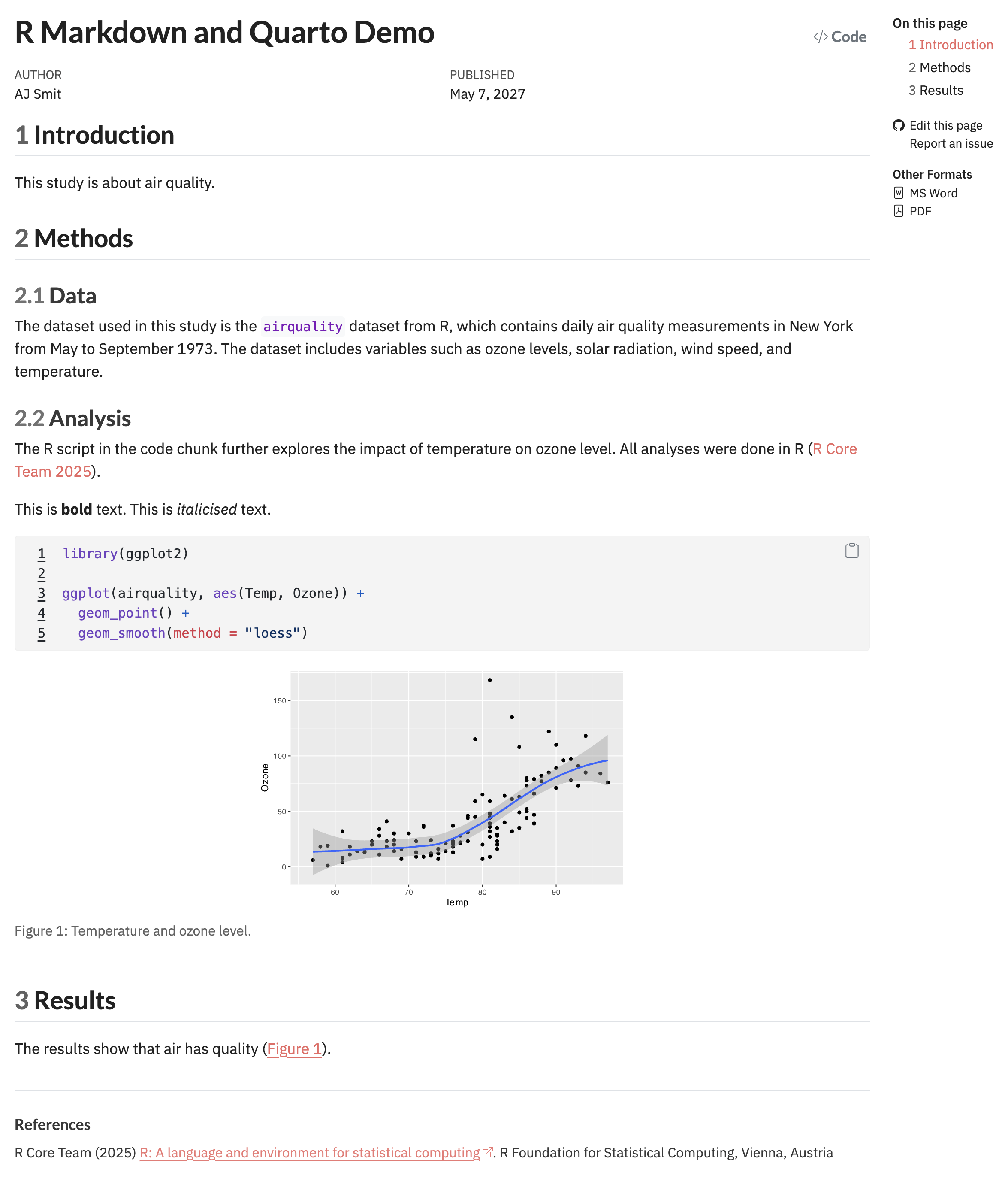
The R script in the code chunk further explores the impact of temperature on ozone level.
All analyses were done in R [@R2025].

This is **bold** text. This is *italicised* text.

```{r}
#| label: fig-airquality
#| fig-width: 6
#| fig-height: 4
#| fig-cap-location: bottom
#| fig-cap: "Temperature and ozone level."
#| warning: false

library(**ggplot2**)

ggplot(airquality, aes(Temp, Ozone)) + 
  geom_point() + 
  geom_smooth(method = "loess")
```

## Results

The results show that air has quality (@fig-airquality).

## Discussion

We used R for the analyses [@R2017]. The results confirm that of Schlegel [-@Schlegel2017].

Notes:

1. Lines 1-14: YAML header
2. Line 16: A level 2 header
3. Line 22: A level 3 header
4. Line 35-48: An R code chunk

In the above example, Lines 1-14 are called the YAML header, which contains metadata about the document. Initially, you’ll not want to include the YAML lines bibliography: ../references.bib and citation: true since you will not have a bibliography file set up yet. The citation: true option is used to enable citations in the document, and you may read more about it elsewhere. A very important part of the YAML header is the statement embed-resources: true which ensures that any images or other resources such as the theming styles etc. used in the document are embedded directly into the HTML output, making it self-contained and portable — this is essential when you want to share your document with others, publish it online, or submit it for grading.

Lines 16-33 are the first two sections (two level one headings, “Introduction” and “Methods”, the latter with two level three headings beneath is, i.e., “Data” and “Analysis”) of the document.

Lines 35-48 make the code chunk, which is where we embed our R code. The #| fig-cap option in the code chunk specifies the caption for the figure that will be generated, and you can cross reference this from the body (see Line 52) text using @fig-airquality — this references the name specified by #| label: fig-airquality. The code chunk itself generates a figure that shows the relationship between temperature and ozone level in the airquality dataset. Notice also how I have cited a reference, @R2025, which is a reference to the R software itself, which is specified in the bibliography file references.bib (which you will need to create in your own time).

ImportantDo This Now

1. Go to the RStudio menu and find ‘File’ > ‘New File’ > ‘Quarto Document’ and create your own Quarto file.
2. Save it using a descriptive name inside of your R Project directory.
3. Copy and paste the example skeleton into your own, fresh Quarto file.
4. Make a few edits to your taste, such as at least changing the author’s name.
5. Render it (via the ‘Render’ button above the Code Editor).

After you’ve rendered this file, you’ll see the following output (the HTML output shown):

The HTML output of the above Quarto document.

3.1 Supported output formats

By changing the format option in the YAML header, you can export your report to different types including:

• PDF documents (provided you have LaTeX installed)
• HTML web pages
• Word (.docx) documents

For example:

format: pdf

or

format: docx

3.2 Rendering the document

• In RStudio or Positron, you can click the ‘Render’ or ‘Preview’ button, respectively, to produce your desired output.
• You can also use the command line: $ quarto render my_file.qmd$

Each time a document is rendered, Quarto re-executes the entire analysis from top to bottom in a clean session. This process tests:

1. whether objects are created in the order you assume,
2. whether variables exist where you think they do, and
3. whether your results really follow from the code as written rather than from residual state in the interactive environment.

So, rendering early and often is a useful and time-saving habit. Errors encountered during rendering are signs that direct you to hidden dependencies, misplaced assumptions about object scope, or inconsistencies between narrative and computation. A plot that appears correctly in the console but fails during rendering may reveal that it relies on objects created interactively rather than within the document itself. Similarly, warnings or failures triggered only at render time frequently indicate that code chunks are implicitly dependent on earlier chunks in ways that are not yet explicit.

Thus, rendering is part of analysis and it brings analytical claims, code structure, and computational order into alignment. Develop the habit of rendering regularly. This helps ensure that your document remains executable, interpretable, and resilient to change. This practice will become increasingly important in later sections of the module, where analyses grow longer. In real life, projects may become more modular, and assumptions that once remained implicit must be made visible and defensible.

You will thank me later for my insistence to perform frequent rendering when it comes to tests and exams!

NoteWhat went wrong?

A common early error occurs when a document that previously rendered successfully begins to fail after a small, seemingly innocent edit to the YAML header. For example, placing a blank line between two entries, or misaligning an option such as format: by a single space, can cause Quarto to misinterpret the document structure. The resulting error messages may be indirect, such as complaints about missing formats, unknown options, or failures later in the render process. This is because the problem does not sit with the analysis, but with how the YAML metadata was parsed.

When this happens, the most effective response is to compare the YAML carefully against a known working example and restore its structural alignment. In practice, many YAML issues are resolved by undoing well-intentioned formatting “tidy-ups” that the parser does not understand.

The restrictions you encounter here (minimal YAML headers, limited citation use, and carefully staged document structure) are not endpoints. The are the framework. In later sections of the module, these same elements are revisited and extended: bibliographies and cross-referencing become central to statistical reporting, YAML options expand document capabilities and format, and Quarto documents evolve from simple reports into modular, project-level artefacts.

4 More Detailed Information

Please refer to the Markdown Basics page on the Quarto website for much more information about Markdown.

Quarto is extremely powerful and you’ll want to explore the Markdown Basics page thoroughly in your own time. Of immediate interest to most of you will be the page on Citations, or the other information under “Authoring” that you may access on the Quarto Guide.

You will also have to explore the various YAML options. You can specify these at the beginning of your document in the YAML block at the top, which allows you to define various options for how your HTML, Word document, PDF, or any of the many formats that Quarto can produce, will look. Please consult the reference section on the Quarto website for the various YAML options available (e.g., here the HTML YAML options), so that you can set up your document in the way you would like it to appear.

Be reminded that YAML is very particular about the way the various levels of indentation must appear in order for the it to be read correctly by your Quarto system and for the code to execute correctly. So, this is an excellent opportunity for you to pay attention to detail and ensure that your YAML is precisely structured according to the expectations of the example document provided.

5 Reproducibility as Practice

Reproducibility, in the context of Quarto and R Markdown, is a disciplined workflow. Quarto supports reproducible analysis by requiring that code, narrative, and outputs be generated together from a single source document, and so reduces the scope for undocumented intermediate steps or post hoc modification of results. When a document is rendered, all analyses are re-executed in sequence, forcing dependencies, object creation, and analytical order to be made explicit. This makes hidden assumptions (e.g., about data preparation, parameter choices, or plotting defaults) visible in a way that conventional copy-and-paste workflows do not.

At the same time, reproducibility remains contingent. It depends on stable input data, explicit control of randomness, and awareness of the computer system on which the document is rendered. Quarto does not freeze package versions, manage software dependencies, or archive external data sources on your behalf (but you can make it do so with some know-how). It provides instead a structured setting in which such practices can be adopted consistently. So, Quarto should be seen as an enabling infrastructure… it makes reproducible work tractable, inspectable, and shareable, but it does not absolve the user from methodological responsibility. Treating reproducibility as an active practice (one that must be maintained rather than assumed) is implicit to using Quarto well.

We will cover reproducibility in some more detail under section 2. Working with Data & Code.

6 Why Use R Markdown?

Using R Markdown within Quarto allows your analysis to be conducted, documented, and communicated within a single, coherent structure. Data preparation, statistical analysis, figures, and interpretation are written together, rather than assembled after the fact from disconnected sources or from memory. This integration makes analytical decisions visible and obvious, both to others and to yourself when you return to the work weeks or months later. Because results are regenerated directly from code at render time, documents remain reusable: the same analysis can be re-run on updated data, revised parameters, or alternative subsets without reconstructing the surrounding narrative. These properties will become increasingly important in the next chapter, where we shift from individual scripts to project-based workflows and begin treating analyses as evolving objects rather than one-off tasks.

The value of this approach becomes clearer when compared to a more ad-hoc way of working. Think about an analysis in which data are cleaned interactively in the console (or, shock-horror, in a spreadsheet!), figures are produced through incremental trial-and-error, and only the final plots are copied into a word processor alongside earlier descriptions of what was done. In such cases, the analytical pathway exists mostly in the user’s memory. Intermediate decisions are discarded and reproducing the analysis (even by the original author) requires reconstruction rather than execution. Small changes in data or software can change results without leaving an obvious trace and make it difficult to diagnose differences or defend analytical choices.

The table below summarises these contrasts schematically:

Aspect	Quarto-based workflow	Ad-hoc workflow
Code and narrative	Written together in a single source document	Separated across scripts, consoles, and documents
Generation of results	Re-executed automatically on render	Manually copied and pasted
Analytical order	Explicit and enforced	Implicit and often undocumented
Reuse with new data	Straightforward re-rendering	Requires partial or full reconstruction
Transparency	Decisions visible in code	Decisions inferred after the fact
Suitability for collaboration	High	Limited

Quarto-oriented workflows are also designed to align smoothly with the material introduced later on workflow management and version control. When analyses live inside a structured project directory and are written as executable documents, they can be tracked over time using tools such as Git, which record how files change rather than just storing their older versions and their final state. You do not need to master version control immediately for this to be useful. Even a basic awareness that your analysis has a history (that it can be inspected, compared, and, if necessary, revisited) reinforces good analytical habits. Reproducibility now extends beyond the moment of rendering a document. It becomes a property of the entire analytical lifecycle, linking day-to-day coding practice with longer-term standards of transparency and accountability that underpin credible quantitative work.