
| Replicate | Light (μmol photons m⁻² s⁻¹) | Photosynthesis (mg C m⁻² h⁻¹) | |
|---|---|---|---|
| 3 | 1 | 100 | 4.59 |
| 17 | 2 | 200 | 8.83 |
| 53 | 5 | 200 | 8.05 |
| 44 | 4 | 350 | 12.27 |
| 35 | 3 | 500 | 12.57 |
| 54 | 5 | 250 | 9.38 |
| 34 | 3 | 450 | 11.90 |
| 11 | 1 | 500 | 13.53 |
| 27 | 3 | 100 | 4.20 |
Lecture 6: Pigments & Photosynthesis
Theory
TipThis Theory Accompanies the Following Lab
1 Introduction: Pigments and Photosynthesis
Good morning everyone, welcome back to BDC223. Today we are going to follow on from our lectures on light, and we are going to be talking about pigments and photosynthesis. Much of today’s discussion, and also the next couple of lectures about pigments as well as chromatic adaptation, is based on two papers I need you to read. The papers are both on iKamva; you can find them there. Please read them while working through these lectures — it is quite important that you understand their content. Everything I am going to talk about today will be explained in a lot greater detail in those two papers.
2 Overview of Pigments in Photosynthetic Organisms
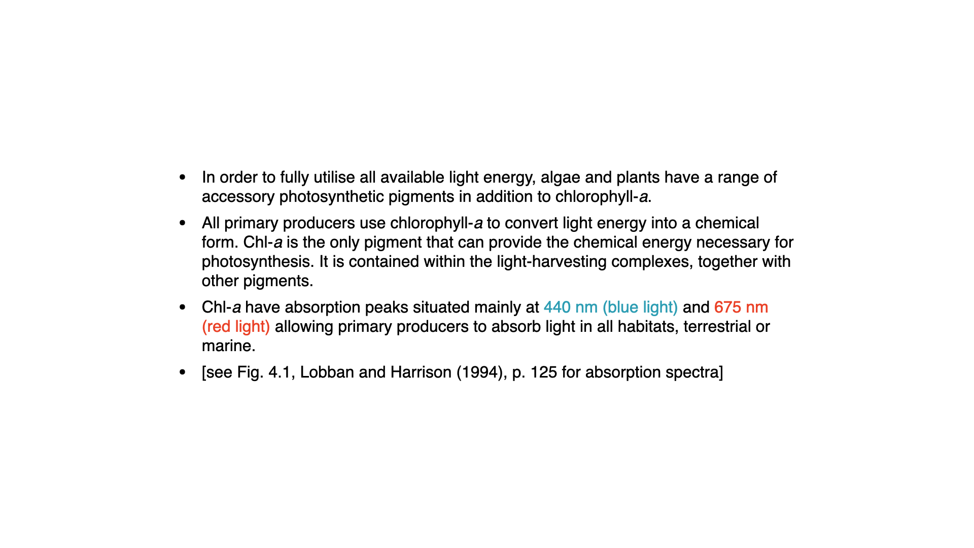
So, in order to exploit the light available in the environment, plants and algae — indeed, all photo-oxygenic organisms — rely on a range of pigments that extract energy from light and convert it into chemical potential energy in the process of photosynthesis.
The predominant pigment in all photo-oxygenic production on Earth, and in all plants, algae, and cyanobacteria, is a molecule called chlorophyll-a. The chlorophyll-a pigment takes light energy and converts it into chemical energy. It is the only pigment that plays such a central role in photosynthesis. There are many other pigments called accessory pigments; they do not directly drive photosynthesis but support light harvesting.
3 Absorption Properties of chlorophyll-a and Accessory Pigments
Chlorophyll-a absorbs light mainly in the blue and red regions. In the previous lecture you saw that visible light falls between roughly \(390\) nm to around \(760\) nm. That is the range of photosynthetically active radiation. However, within that range, not all light is equally effective at driving photosynthesis. This is because chlorophyll-a can maximally absorb light at \(440\) nm (blue light) and \(675\) nm (red light).
Regardless of where these primary producers are — on land, in water, or elsewhere — they are sensitive to blue and red light. If they do not have sufficient light at precisely those wavelengths, their rate of photosynthesis will be impaired.
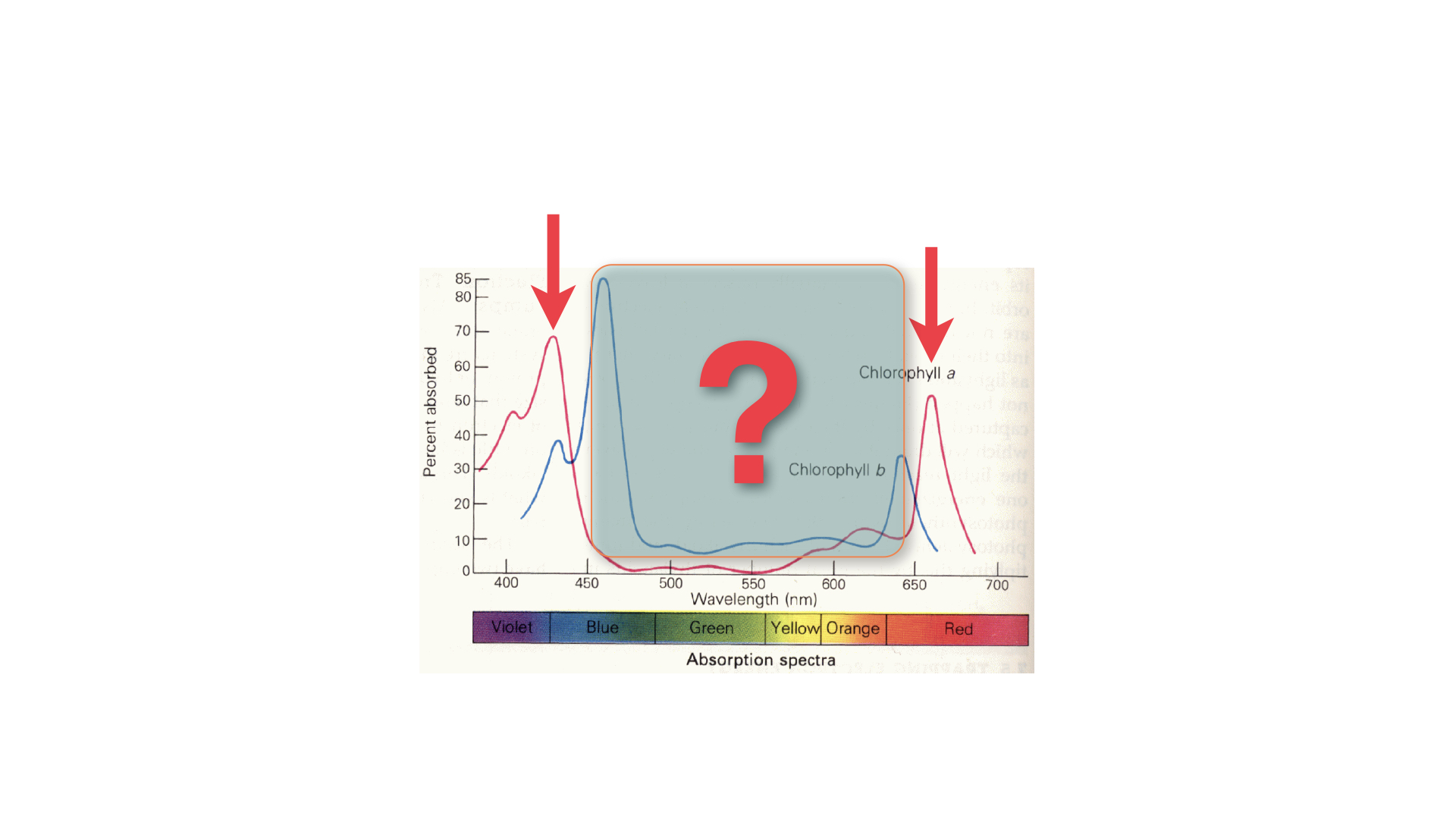
Here are some graphs (Slide reference) that show the absorption for chlorophyll-a and chlorophyll-b. chlorophyll-a, shown as the red line, has two main peaks: one around \(425\) nm (blue) and one in the red region around \(660\) to \(675\) nm. Chlorophyll-b has similar peaks but they are shifted: the blue peak sits nearer to \(460\) nm, closer to green, and the red peak falls slightly toward the orange region.
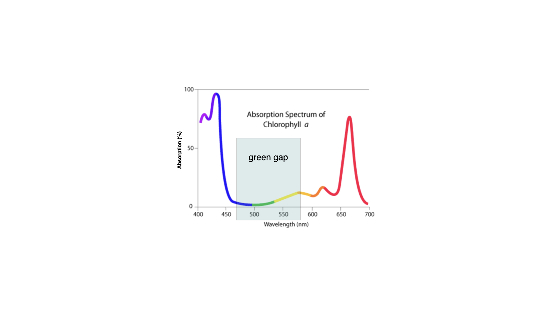
Chlorophyll-b (in fact, none of the accessory pigments) does not drive photosynthesis directly, but it can harvest light and pass that energy to chlorophyll-a, thus broadening the range of light absorbed and utilised for photosynthesis. You will notice that, in the middle of these spectra, there is a gap — a region where light is available yet not absorbed by chlorophyll-a or b. This is often referred to as the “green gap” and is the reason why plants appear green: green light is not absorbed by the major photosynthetic pigments in most leaves, so it is reflected back into the environment and to our eyes.
NoteHow Do Accessory Pigments Pass on Energy to the Reaction Centers?
Accessory pigments transfer the energy they capture from light to chlorophyll-a through a mechanism known as resonance energy transfer (more precisely, Förster resonance energy transfer, or FRET, in biophysical terms). This is a non-radiative process, meaning that the energy is not emitted as light and then reabsorbed, but is instead conveyed directly through electromagnetic interactions between the excited accessory pigment and the chlorophyll-a molecule. When a photon excites an accessory pigment, its electrons are elevated to a higher energy state; as this energy relaxes, it is transferred to a neighbouring chlorophyll-a molecule if the two pigments are sufficiently close (usually within 2–6 nanometres) and their electronic energy levels are appropriately aligned. At distances below ~1–2 nanometers, excitonic coupling can take place, wherein the excited states of neighbouring pigments become quantum-mechanically delocalised across multiple molecules rather than localising on discrete donors and acceptors.
The thylakoid membrane in chloroplasts is not a disordered soup of pigments but a carefully arranged molecular architecture known as the light-harvesting complex (LHC). Within these complexes, accessory pigments (such as chlorophyll-b and various carotenoids) are embedded in protein scaffolds alongside chlorophyll-a in spatial configurations that maximise energy transfer efficiency. The proteins hold pigments at precise orientations and distances that facilitate resonance coupling between excited states. The energy “hops” from pigment to pigment down an energetic gradient, ultimately funnelling to the reaction centre chlorophyll-a, where the photochemical conversion (electron transfer) occurs. This funnel-like arrangement of pigments and the efficiency of resonance transfer together allow plants and algae to capture a broad spectrum of solar radiation and direct it toward the relatively narrow photochemical core without significant loss.
4 The Green Gap and Accessory Pigments
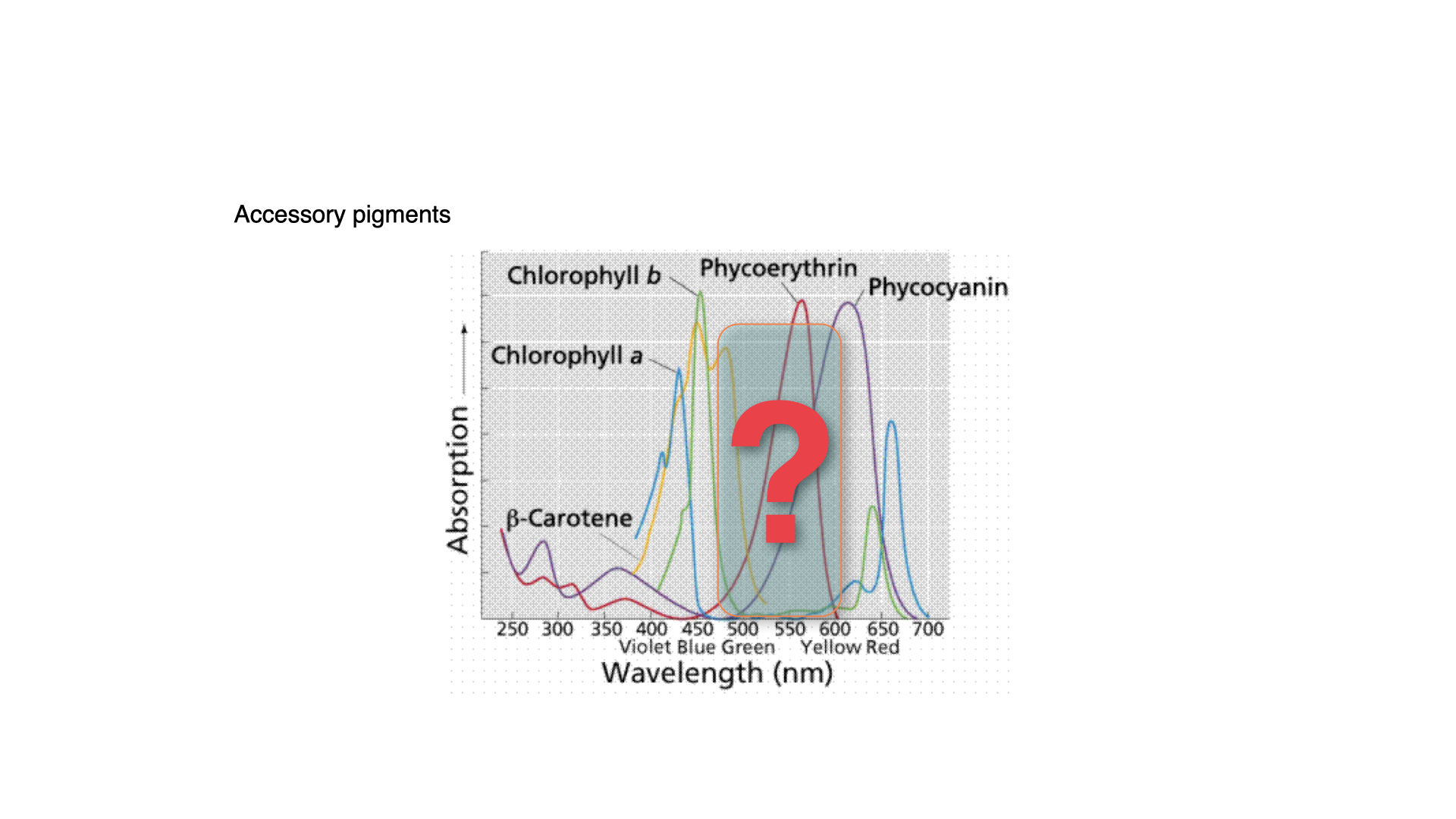
Plants have evolved various pigments to fill that green gap. Among the most notable of these are carotenoids, which include beta-carotene, and the phycobilins, such as phycoerythrin and phycocyanin. Carotenoids are also the pigments responsible for the orange colour in carrots, as indicated by the orange line on many absorption spectra.
The carotenoids and phycobilins absorb light in the green gap and pass that energy on to chlorophyll-a, enabling photosynthesis that would otherwise not occur at those wavelengths. These are called accessory pigments because they complement the absorption range of chlorophyll-a and make photosynthesis more effective in sub-optimal light conditions.
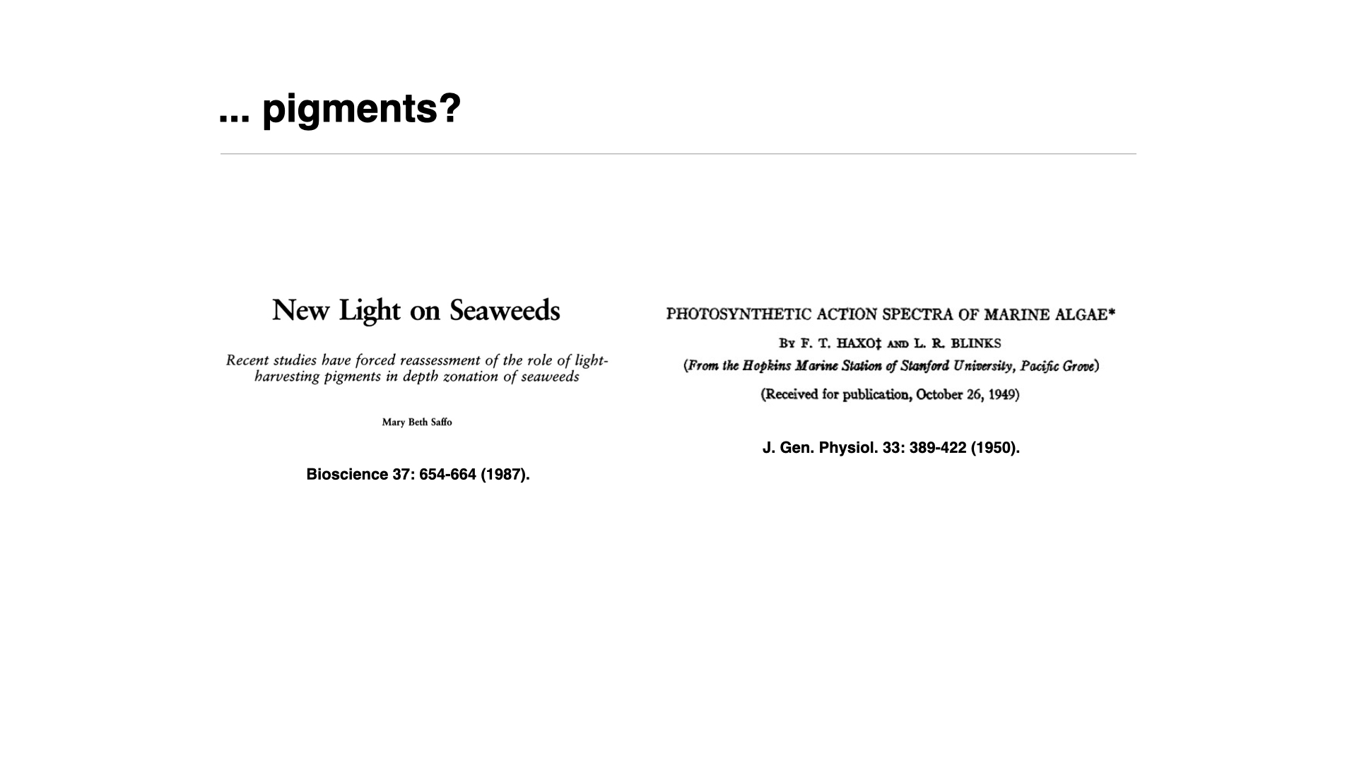
At first glance, the diversity of accessory pigments appears as vast as the diversity of light climates in the ocean, on land, and in freshwater. However, later experiments — especially those by Engelman, Haxo, and Blinks (to be discussed in your papers)—demonstrate that the diversity of accessory pigments does not necessarily correspond to the diversity of environmental light conditions.
5 Classification and Function of Pigments
There are three main pigment classes:
- Chlorophylls – The major photosynthetic pigments. chlorophyll-a is primary, with chlorophylls-b and -c acting as accessory pigments that transfer absorbed energy to chlorophyll-a.
- Carotenoids – Includes beta-carotene and xantho-phylls, which also serve as accessory pigments.
- Phycobilins – Reddish or purplish pigments, including phycocyanin and phycoerythrin, mainly found in certain algae and cyanobacteria.
Across all photoautotrophs, there are more than forty pigments involved. They bind differently to the proteins making up the photosynthetic machinery, expanding the plant’s ability to absorb different wavelengths, especially in the green gap, and maintain high photosynthetic efficiency in a range of environments.
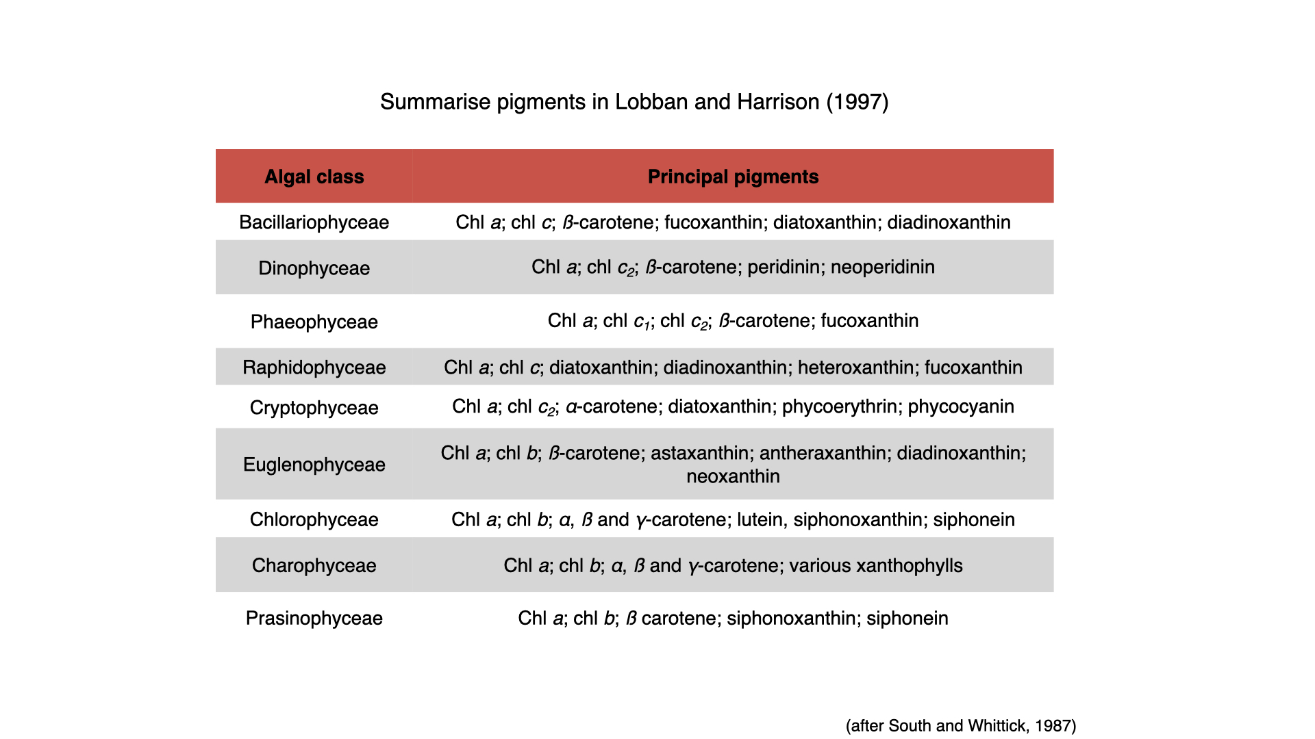
Especially in algae, the types of pigments present can indicate taxonomic relationships and phylogenetic heritage. By extracting pigments from a seawater sample, for example, one can deduce the classes of algae present. Similar underpinnings occur in terrestrial plants, with certain pigments associated with specific plant types.
6 What Is Photosynthesis?
Photosynthesis is the conversion of light energy — radiant energy — into chemical potential energy. It drives carbon fixation: uptake of \(\mathrm{CO}_2\) from the environment, splitting water, and releasing oxygen as a byproduct. The reactions occur in the photosystems I and II.
As a function of light intensity, photosynthesis responds with an increased rate — to a point. This relationship is described by the photosynthesis-irradiance (PI) curve.
7 The Photosynthesis-Irradiance (PI) Curve
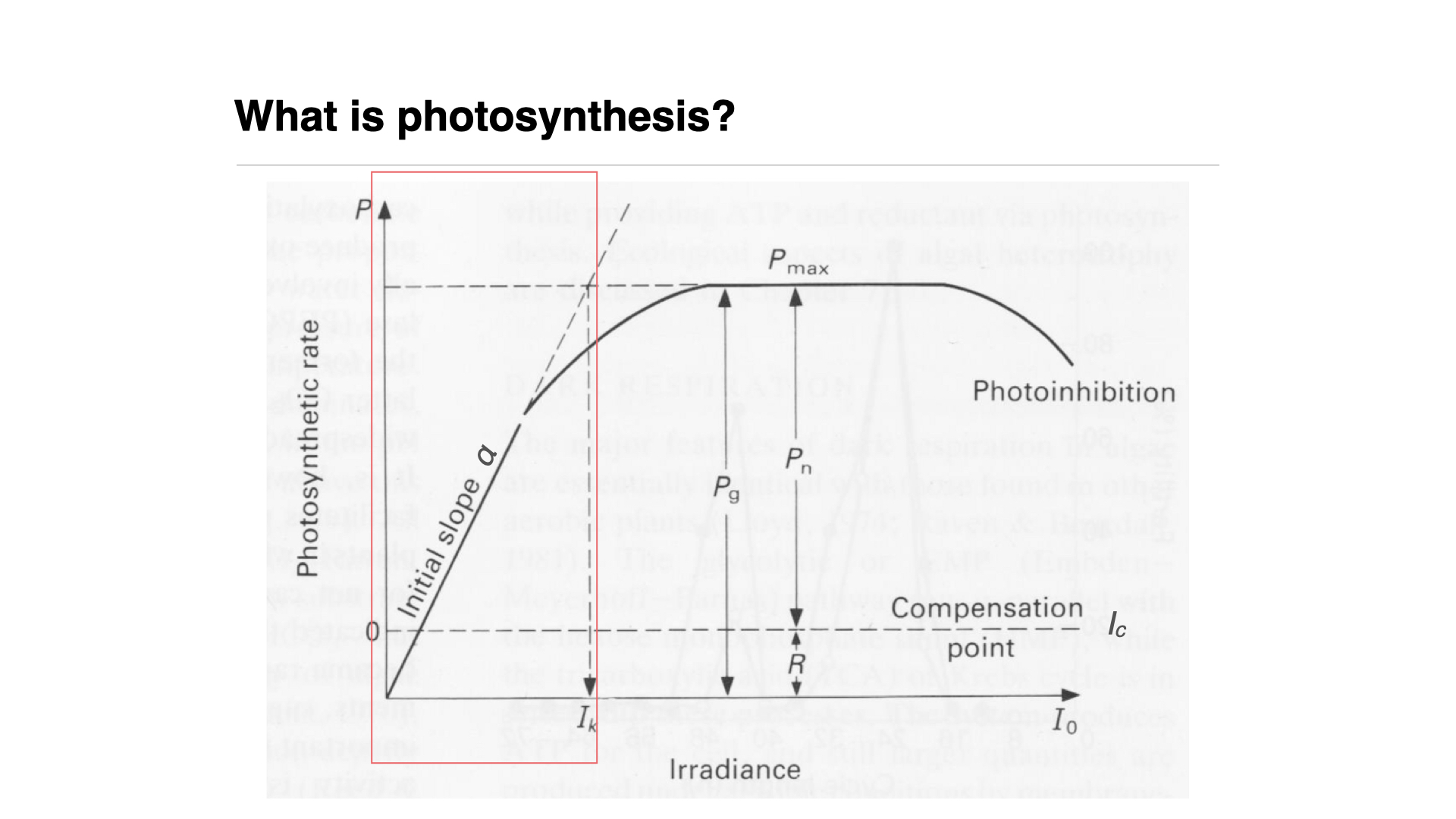
The PI curve (Slide reference):
- Y-Axis: Rate of photosynthesis, measured by carbon incorporation (e.g., mg C m\(^{-2}\) s\(^{-1}\), mg C m\(^{-2}\) hr\(^{-1}\), or mg C m\(^{-2}\) day\(^{-1}\)).
- X-Axis: Irradiance (light intensity).
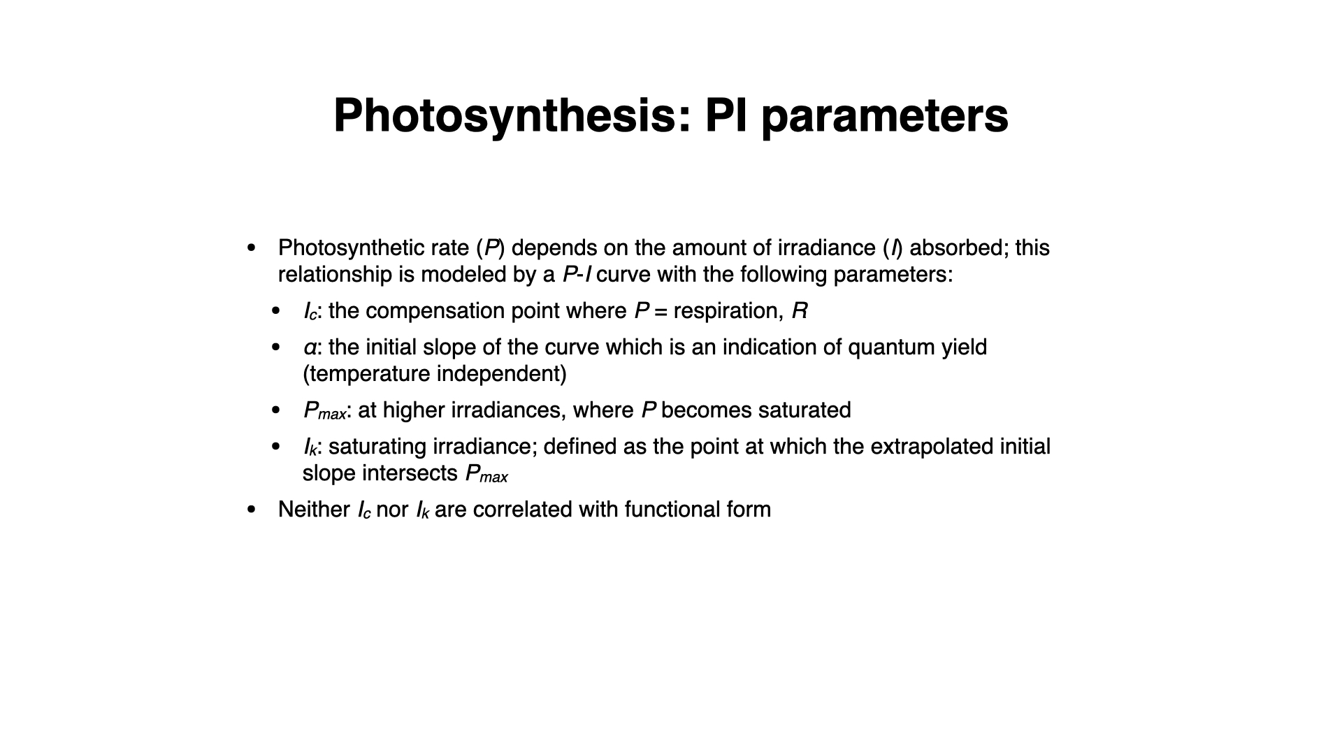
Initially, the PI curve is linear: as irradiance increases, photosynthesis increases at a rate defined by the slope \(\alpha\) (alpha). Alpha reflects the plant’s sensitivity to changes in irradiance. A steep alpha (steep slope) means more sensitivity to small changes in light; a shallow slope indicates less sensitivity and a need for greater changes in light intensity to affect photosynthesis rate.
At a certain point, the rate reaches saturation, denoted as \(I_k\). This occurs where the extrapolated horizontal maximum rate (\(P_{max}\)) intersects with the linear part of the curve. Beyond this, increasing light does not increase photosynthetic rate since all the photosynthetic machinery is working at full capacity — much like pressing a car accelerator to the floor when the engine cannot go faster.
Should irradiance keep increasing, photosynthesis can decline — a phenomenon called photoinhibition. Here, excessive light can cause actual damage, or trigger protective mechanisms within the photosynthetic apparatus to prevent damage, analogous to running a car engine past its operating limits.
Respiration occurs at all times, consuming oxygen, while photosynthesis (in the presence of light) produces it. At low light, the rate of oxygen production by photosynthesis is less than the rate of consumption by respiration, resulting in net negative oxygen production. The light compensation point is the irradiance where net oxygen production is zero.
Net photosynthesis: Above the compensation point — positive net oxygen evolution.
Gross photosynthesis: Total oxygen produced, regardless of respiration.
Understanding these parameters — the light compensation point, \(\alpha\), \(P_{max}\), \(I_k\), etc.—is crucial. We will revisit this concept in practical sessions where you will fit models to real data.
7.1 The hyperbolic tangent model
The hyperbolic tangent model was proposed by Jassby and Platt (1976). It has become one of the most widely used models for describing the relationship between photosynthetic rate and irradiance (light intensity) in aquatic photosynthetic organisms, including algae ranging from kelp to phytoplankton. The model captures the core dynamics of photosynthesis, in which the rate of photosynthesis initially increases with light intensity but eventually saturates as the photosynthetic machinery reaches its maximum efficiency. This is a simple model, but it effective because the biologically meaningful parameters can be directly interpreted to assess plant or algal productivity in various light environments.
The hyperbolic tangent model is expressed as:
\[ P(I) = P_{\text{max}} \times \tanh\left(\frac{\alpha I}{P_{\text{max}}}\right) \]
Where:
- \(P(I)\) represents the photosynthetic rate at a given irradiance \(I\) (light intensity),
- \(P_{\text{max}}\) is the maximum photosynthetic rate (also referred to as the light-saturated rate),
- \(\alpha\) is the initial slope of the curve, which reflects the photosynthetic efficiency at low light levels,
- \(I\) is the irradiance (light intensity),
One is also able to determine the saturating irradiance, \(I_{\text{k}}\), which is the light intensity at which photosynthesis reaches \(P_{\text{max}}\). Simply read this value off the graph where \(P(I) = P_{\text{max}}\) (see the lecture slides ‘6.BDC223_Pigments_Photosynthesis_2024.key.pdf’.
The hyperbolic tangent function \(\tanh\) is used to smoothly describe the transition between the linear increase in photosynthesis at low light intensities and the eventual plateau at higher intensities, where photosynthesis becomes light-saturated. The light compensation point, the point at which photosynthesis equals respiration (i.e., net photosynthesis is zero), can also be derived from this model.
The model describes the essential processes of photosynthesis with just two parameters: \(P_{\text{max}}\) and \(\alpha\). Both parameters are biologically meaningful and tell us how efficiently an organism can convert light into chemical energy under different light conditions. For example, higher values of \(P_{\text{max}}\) indicate a greater potential for photosynthesis under optimal light conditions, while the value of \(\alpha\) indicates how quickly photosynthesis responds to low light.
Applications of the hyperbolic tangent model are numerous. It is commonly used to estimate the photosynthetic performance of marine and freshwater algae, seagrasses, and macroalgae under varying environmental conditions. In kelp forests, for instance, we may use this model to assess how different species adapt to light intensities at various depths or how photosynthetic performance shifts in response to seasonal changes in light availability. Looking at phytoplankton, the model helps estimate productivity across different layers of the water column, where light intensity decreases with depth.
Below are a few lines of data taken from a hypothetical P-I experiment. The data are for five replicate experiments with the same light intensities (independent variable), representing conditions typically encountered by kelp at latitudes between -36° and -23°S.

After fitting the model to the data, we can determine the values for \(P_{\text{max}}\) and \(\alpha\) for each replicate and determine the average value across the five fits. The combined plot (Figure 1) displays the observed data points for all replicates and the fitted curve from the first replicate.
The average model fit values of the estimated parameters across all replicates are as follows:
- \(P_{\text{max}}\): 13.05 mg C m⁻² h⁻¹
- \(\alpha\): 0.05 μmol photons m⁻² s⁻¹
7.2 Considering the light compensation point
The light compensation point (\(I_c\)) is the irradiance level at which the rate of photosynthesis equals the rate of respiration, resulting in a net photosynthetic rate of zero. Below this point, the organism consumes more energy (via respiration) than it produces through photosynthesis, leading to a net loss of energy. Estimating \(I_c\) is important for determining the minimum light intensity required for the survival of photosynthetic organisms, after compensation for the effect of cellular respiration.
In the context of the Jassby and Platt hyperbolic tangent model, \(I_c\) can be estimated by solving for the irradiance \(I\) when the net photosynthetic rate \(P(I)\) equals zero:
\[ 0 = P_{\text{max}} \times \tanh\left(\frac{\alpha I_{\text{LCP}}}{P_{\text{max}}}\right) \]
Since \(\tanh(0) = 0\), the net photosynthetic rate is zero when \(I = 0\). However, due to respiration, the net photosynthesis can be negative at zero light intensity. To account for respiration, we can modify the model to include dark respiration rate (\(R\)):
\[ P(I) = P_{\text{max}} \times \tanh\left(\frac{\alpha I}{P_{\text{max}}}\right) - R \]
Now, \(I_c\) is the irradiance at which \(P(I) = 0\):
\[ 0 = P_{\text{max}} \times \tanh\left(\frac{\alpha I_{\text{LCP}}}{P_{\text{max}}}\right) - R \]
We can solve this equation numerically to find \(I_{\text{LCP}}\).
| Replicate | Light (μmol photons m⁻² s⁻¹) | Photosynthesis (mg C m⁻² h⁻¹) | |
|---|---|---|---|
| 3 | 1 | 100 | 3.65 |
| 37 | 4 | 0 | -2.17 |
| 5 | 1 | 200 | 6.98 |
| 57 | 5 | 400 | 9.43 |
| 54 | 5 | 250 | 7.41 |
| 60 | 5 | 550 | 10.98 |
| 33 | 3 | 400 | 9.66 |
| 6 | 1 | 250 | 7.89 |
| 49 | 5 | 0 | -1.86 |

The model fit to the data is in Figure 2. The average model fit values of the estimated parameters across all replicates are as follows:
- \(P_{\text{max}}\): 13.15 mg C m⁻² h⁻¹
- \(\alpha\): 0.05 μmol photons m⁻² s⁻¹
- \(I_c\): 41.28 μmol photons m⁻² s⁻¹
7.3 Platt et al. (1980) model with photoinhibition
Let us now look at the Platt et al. (1980) model, which incorporates photoinhibition into the photosynthesis-irradiance (P-I) relationship. This model extends the understanding of photosynthesis by accounting for the decrease in photosynthetic efficiency at high light intensities due to photoinhibition — a phenomenon where excessive light damages the photosynthetic apparatus, leading to reduced photosynthetic rates.
The model is expressed mathematically as:
\[ P(I) = P_{\text{max}} \left(1 - \exp\left(-\frac{\alpha I}{P_{\text{max}}}\right)\right) \exp\left(-\frac{\beta I}{P_{\text{max}}}\right) \]
Where:
- \(P_{\text{max}}\) is the maximum photosynthetic rate in the absence of photoinhibition.
- \(\beta\) is the photoinhibition parameter (rate of decrease in photosynthesis at high light).
- \(\exp\) denotes the exponential function.
This model combines the positive effect of light on photosynthesis at low irradiance with the negative effect of photoinhibition at high irradiance, providing a comprehensive description of the photosynthetic response across a wide range of light intensities.
| Replicate | Light (μmol photons m⁻² s⁻¹) | Photosynthesis (mg C m⁻² h⁻¹) | |
|---|---|---|---|
| 45 | 3 | 1000 | 10.05 |
| 76 | 5 | 700 | 9.13 |
| 34 | 2 | 1600 | 10.16 |
| 52 | 4 | 0 | -2.00 |
| 1 | 1 | 0 | -0.86 |
| 77 | 5 | 800 | 9.58 |
| 10 | 1 | 900 | 11.26 |
| 13 | 1 | 1200 | 11.43 |
| 39 | 3 | 400 | 7.98 |

8 Effects of Environmental Stress
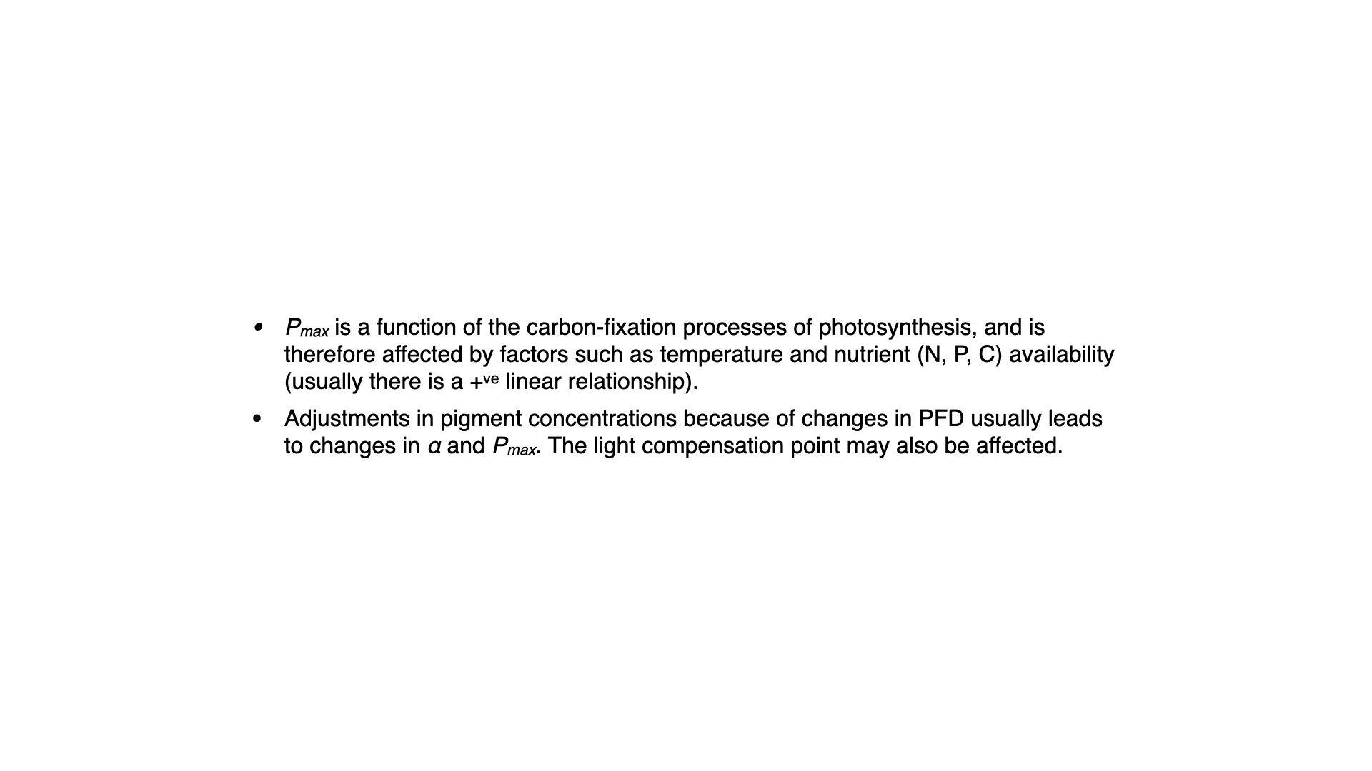
\(P_{max}\) represents the maximum photosynthetic capacity, which is influenced by many stresses, including thermal stress, nutrient stress, and light stress. Any of these can reduce a plant’s capacity to sustain \(P_{max}\), and a reduction in this parameter is often the first sign of environmental stress. Measuring these rates gives insights into how and when plants become stressed.
Here are some indicative values (Slide reference):
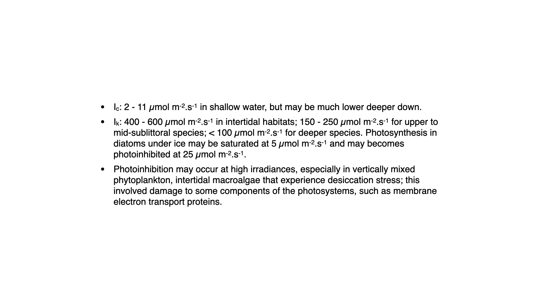
- Intertidal environments: light saturation might occur at \(400\)–\(600\;\mu\mathrm{mol}\,\mathrm{m}^{-2}\,\mathrm{s}^{-1}\)
- Sublittoral species (deeper): saturated at \(150\)–\(250\;\mu\mathrm{mol}\,\mathrm{m}^{-2}\,\mathrm{s}^{-1}\)
- As depth increases, saturation occurs at progressively lower irradiances.
- Some deep-water plants can become photoinhibited at what would seem to us like relatively dim light.
These values—\(I_C\), \(I_K\), \(P_{max}\), \(\alpha\)—vary among species, being determined both by environmental adaptation and genetic heritage, and thus serve as good indicators of a plant’s typical habitat and stress response.
What we saw above is a standard textbook interpretation and formulation of a PI-curve. However, there are several mathematical models that can be used to describe the PI-curve. We will look at two of the most commonly used models: the hyperbolic tangent model by Jassby and Platt (1976) and the Platt et al. (1980) model, which includes photoinhibition.
9 Absorption Spectrum Vs Action Spectrum
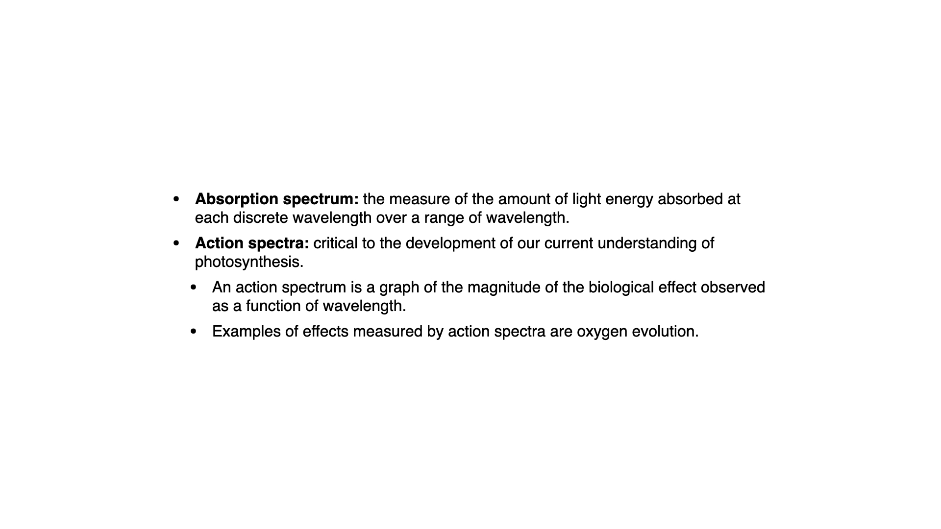
Before moving on, it is critical to distinguish the absorption spectrum from the action spectrum.
- Absorption spectrum: Measures the amount of light absorbed by all pigments at every wavelength — essentially, how much light is not reflected or transmitted.
- Action spectrum: For each wavelength, measures the biological effect — oxygen evolution rate — that results from absorption.
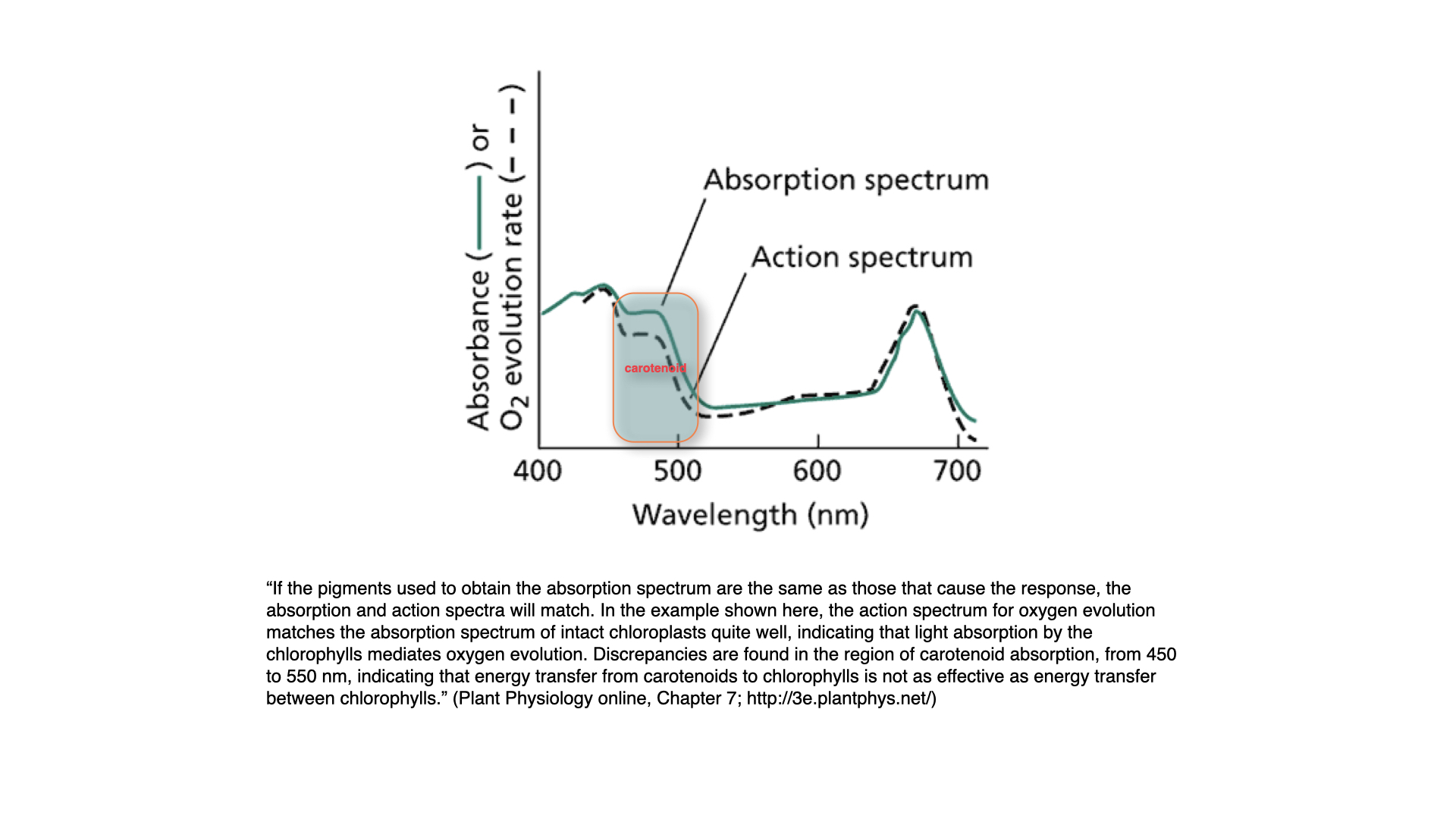
Typically, the action and absorption spectra match well, but not perfectly. For instance, between about \(450\) and \(500\) nm, there is a mismatch. This occurs because, beyond the optimal absorption peak of chlorophyll-a, carotenoids start absorbing light. While they can capture light within this region, they are less efficient at passing the energy to chlorophyll-a, resulting in a lower action than absorption value.
This demonstrates that the ability of accessory pigments to pass energy to chlorophyll-a is not perfectly efficient; some energy is lost in the process. Nonetheless, the presence of carotenoids extends the range in which photosynthesis can be driven by chlorophyll-a.
In summary, accessory pigments are essential in harvesting a broader range of light and making photosynthesis effective under varied light environments, even if energy transfer from accessory to primary pigments is not perfectly efficient.
Reuse
Citation
BibTeX citation:
@online{smit2026,
  author = {Smit, A. J. and J. Smit, A.},
  title = {Lecture 6: {Pigments} \& {Photosynthesis}},
  date = {2026-03-19},
  url = {https://tangledbank.netlify.app/BDC223/L06-pigments_photosynthesis.html},
  langid = {en}
}
For attribution, please cite this work as:
Smit AJ, J. Smit A (2026) Lecture 6: Pigments & Photosynthesis. https://tangledbank.netlify.app/BDC223/L06-pigments_photosynthesis.html.