Lecture 8a: Nutrient Uptake
Uptake Theory

Nutrient uptake, Michaelis-Menten kinetics, Algal nutrition
1 Introduction: the Centrality of Nitrogen
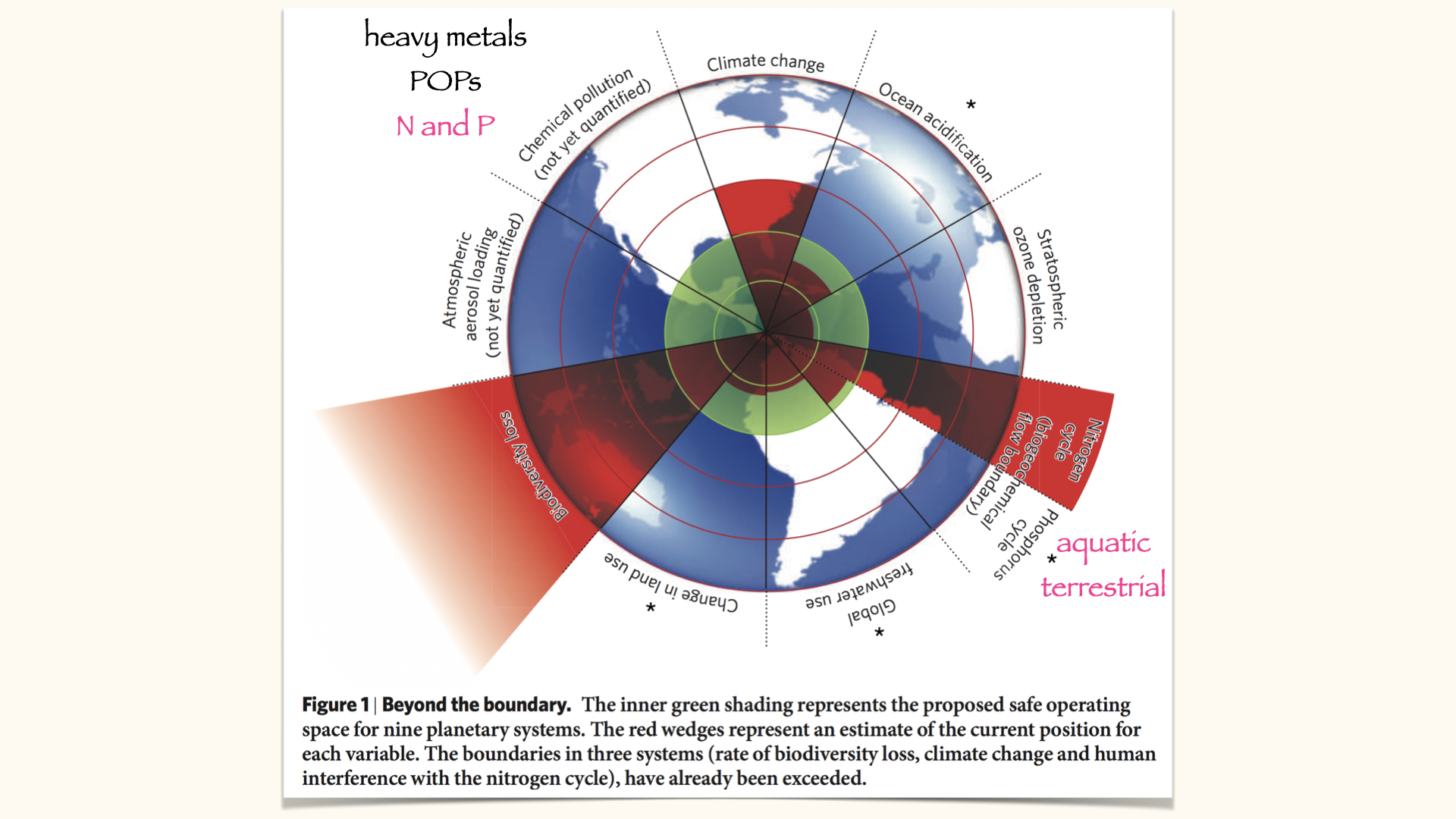
Today’s lecture is centred on the topic of nutrient uptake. We are using nitrogen as our principal example, given its status as a ubiquitous nutrient, essential to all plants for successful growth. Additionally, we will be considering the environmental consequences of there being excessive nitrogen in the environment. This is tied directly to the planetary boundaries concept expounded by Johan Rockström, specifically the quadrant concerning the nitrogen and phosphorus cycles — two key global biogeochemical cycles involving the transportation and transformation of these elements between the biosphere, geosphere, atmosphere, and oceans.
Nitrogen is a particular concern, as it is one of the major thresholds humanity has already exceeded globally. This excess results in numerous environmental problems, especially where processes involve plants — primarily aquatic and marine plants, although to a lesser extent, it does impact certain terrestrial plants as well.
1.1 Nitrogen in the environment
Nitrogen’s importance is clear when you consider its abundant presence. Approximately \(79\%\) of the air we breathe is composed of nitrogen, and it is found in soils, sand, and oceans, where it is accessed by plant roots or available in dissolved form for algae and marine plants. The most productive patches of green — on land and visible as blooms in the ocean — are areas of high nitrogen availability, where lush plant and algal growth is possible.
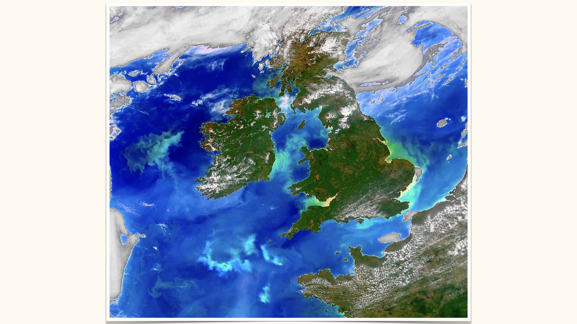
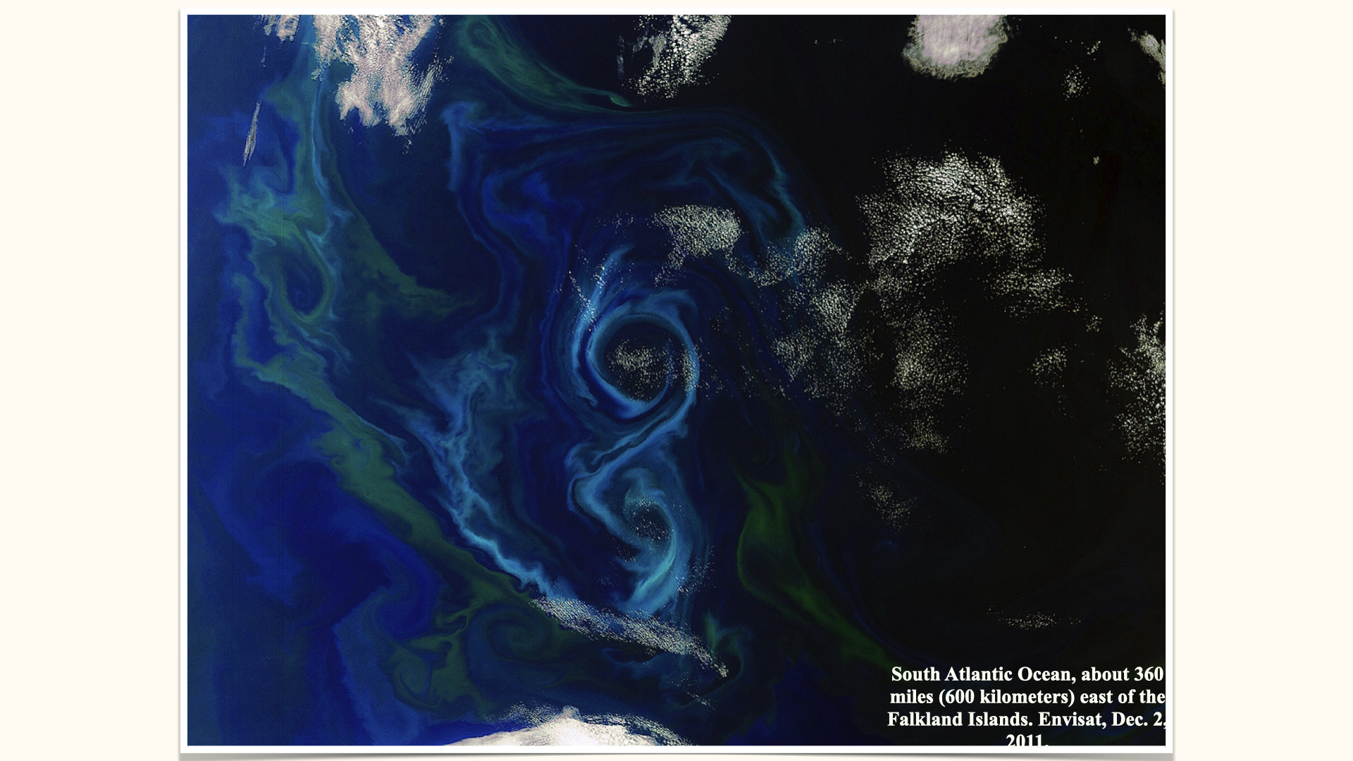
For this module, whilst terrestrial plants will feature in our discussions, our focus throughout the examples will be on aquatic environments, with particular attention to nitrogen dissolved in seawater and its role in triggering phytoplankton blooms. These can be so prolific that they are visible from space — swirls and green patches near the UK, Ireland, or east of the Falkland Islands, all testify to high concentrations of phytoplankton supported by nitrogen availability.
The twirling and swirling patterns you observe in satellite imagery arise from physical ocean mixing processes — currents, eddies — distributing dissolved nitrogen, which in turn supports phytoplankton blooms.
1.2 Environmental consequences of excess nitrogen
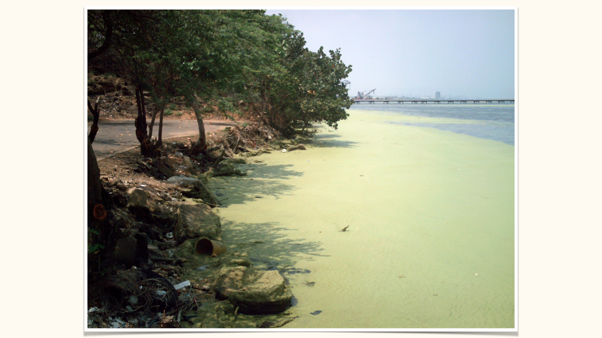
As I have mentioned, excess nitrogen in the environment, from pollution, sewage, or runoff from fertilisers, contributes to unsightly and sometimes malodorous nuisance algal blooms. These blooms are ecologically damaging, reduce water quality, and negatively affect ecosystems and human livelihoods. They are typically accompanied by visible pond scum, floating litter, and other environmental degradation.
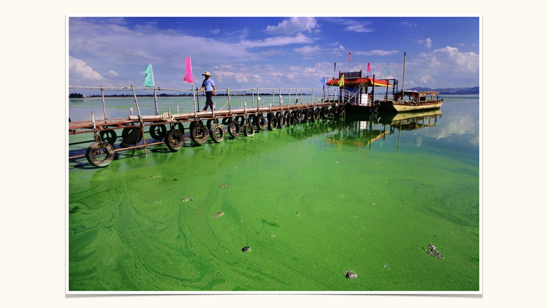
For instance, in China, the large population density and the dispersal of untreated sewage directly into water bodies has led to massive blooms of phytoplankton. Later in the lecture, we will discuss the process of eutrophication, which explains in detail how these blooms develop.
Additionally, certain bacteria, such as photosynthetic cyanobacteria (“blue-green algae”), are part of the problem. As blooms expand, they block light, darkening the water and, through their respiration (especially at night), use up oxygen. Upon death, bacteria decompose the overwhelming biomass, a process which consumes even more oxygen and releases large amounts of \(\mathrm{CO}_2\). The result — known as a dystrophic or anoxic event — is hypoxia or complete anoxia, which leads to further die-offs, especially of aquatic animals requiring oxygen. The largest consumer of oxygen here is the decomposition of dead organic material by bacteria through respiratory processes.
2 Understanding Nutrients and Their Uptake
2.1 What makes a nutrient essential?
Nutrients, alongside light, oxygen, and carbon dioxide, are required for plant and algal growth. In aquatic environments, algae absorb dissolved nutrients directly from the surrounding water. Terrestrial plants usually acquire them through roots in the soil.
Algae, because of their immersion, do not require roots. Their entire body (the “thallus”) is bathed in nutrients. By contrast, plants depend on root systems both for nutrient uptake and for transport to other parts of the organism. You should recall from previous modules how the surface area to volume ratio becomes decisive for nutrient uptake efficiency, particularly in aquatic environments where mixing is driven by environmental processes.
Symbiotic relationships
Terrestrial plants often benefit from symbiotic relationships with fungi and bacteria — mycorrhizae and root nodules — helping them acquire and process nutrients from the soil. Aquatic algae generally do not require such associations, although bacteria in the marine environment do help make nitrogen available for algal uptake.
Bacteria, in terms of both biomass and individual numbers, are among the planet’s most abundant organisms; without them, no form of life would exist.
3 “Taxonomies” of Nutrients
Nutrients can be classified in various ways.
3.1 Essential vs beneficial
Our current understanding of plant nutrient uptake is largely indebted to studies conducted between the 1930s and 1970s. Algae, because of their direct exposure to dissolved nutrients, provided a simple and convenient model to study the principles of nutrient uptake, eventually informing our understanding of the entire plant kingdom.
3.2 A classification based on physiological effect
3.3 Classification informed by nutrient quantities
Essential versus beneficial nutrients: Essential nutrients are those without which a plant cannot survive or complete its life cycle. Even the absence of a single essential nutrient will halt growth, productivity, or reproduction. Beneficial nutrients enhance or facilitate physiological processes, but are not strictly required for survival or completion of the life cycle.
- By Epstein’s (1972) definition, a nutrient is essential if the plant cannot complete a normal life cycle without it, and the element forms part of an essential plant constituent (e.g., magnesium in chlorophyll a).
- Essential nutrients cannot be substituted by another element and must have a direct effect, not just act as a cofactor.
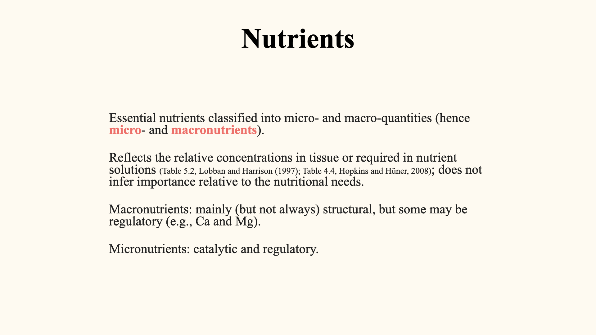
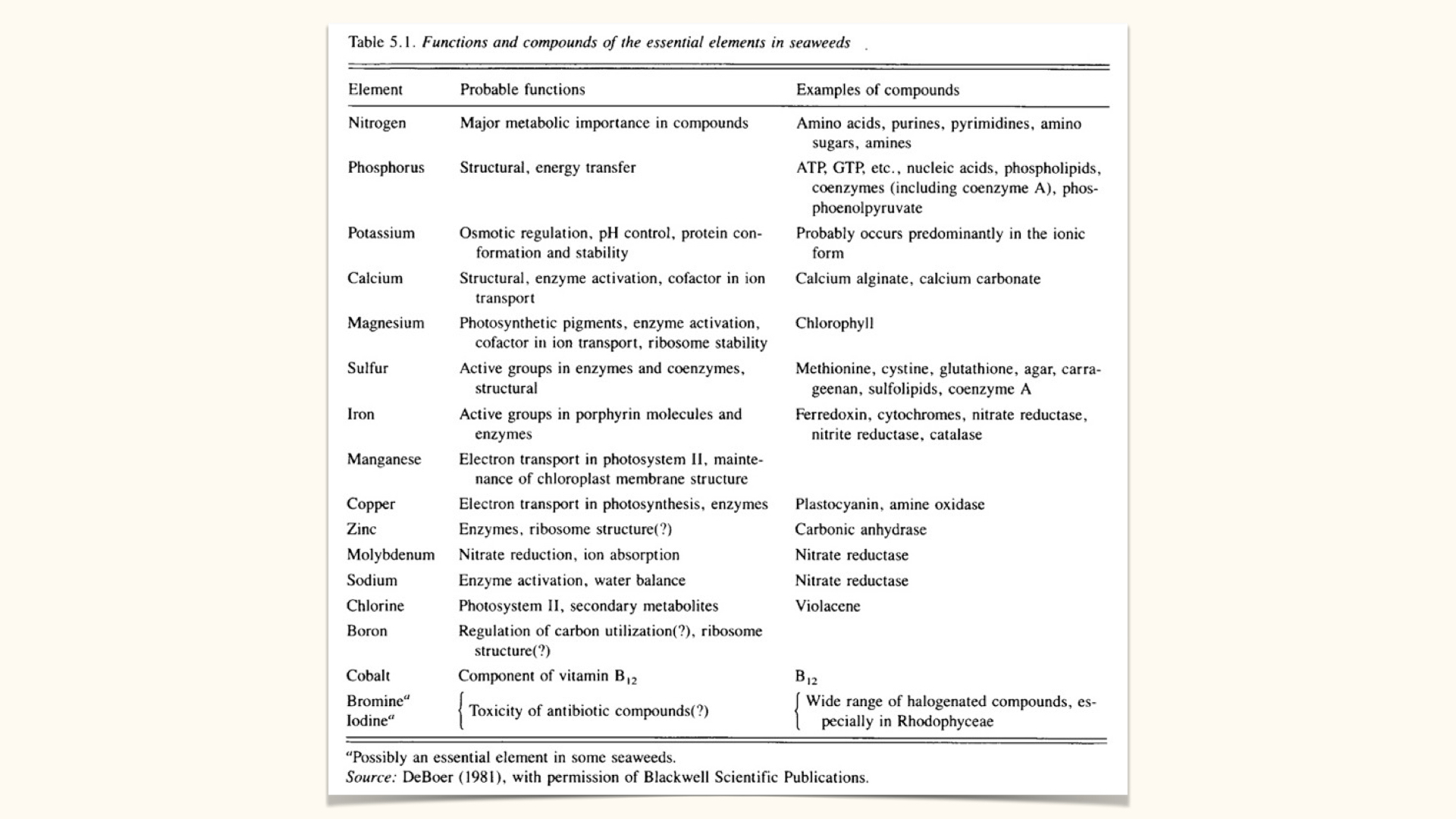
Macronutrients versus micronutrients: This classification reflects the relative quantity needed by the plant. Macronutrients are present and required in much higher concentrations; their roles are often structural, contributing to the biomass of the plant (e.g., carbon, nitrogen, phosphorus, oxygen, potassium). Micronutrients, though required in far smaller amounts, function mainly as catalysts or regulators (e.g., iron in nitrate reductase).
4 So, Which Nutrients Are There?
Higher plants and algae share many (most) of the same nutrients, but their concentrations differ. Also, they differ extensively in the types of macromolecules they possess (e.g., secondary metabolites and so on), which causes the list of nutrients and their abundances to differ somewhat between these taxa.
To reiterate: macronutrients contribute substantially to plant structure and biomass, whereas micronutrients are required in small amounts but are still essential because they act in catalytic and regulatory roles.
Algae (seaweeds) require around \(20\) varieties of nutrients, including:
- Nitrogen
- Phosphorus
- Potassium
- Calcium, among others.
Nitrogen is central because it sits in amino acids, proteins, and nucleic acids. Phosphorus is equally important in nucleic acids, membrane phospholipids, and ATP. Potassium and other nutrients have their own structural and physiological roles.
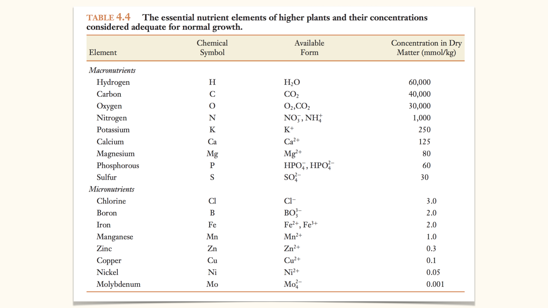
While the precise list of essential nutrients varies modestly between algae and higher plants (the latter require \(17\) essential elements), the principle remains the same: the majority of biomass is composed of macronutrients.
I will not set examination questions that require simple regurgitation of lists (such as “List five essential elements in seaweeds”). Focus, rather, is on understanding the processes and underlying principles.
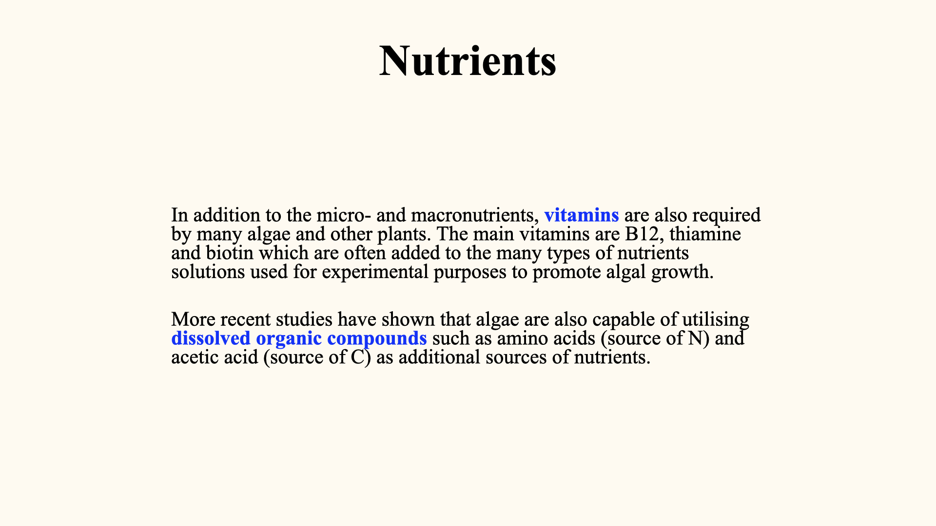
Besides inorganic nutrients (the “bare elements,” not bound in organic molecules), plants can, through mixotrophy, also absorb dissolved organic compounds, though this is much less common and less of a focus for today’s discussion.
5 Concentration Gradients and Uptake Mechanisms
Tables commonly show, per \(\mathrm{kg}\) of dry plant material, that macronutrient concentrations are several orders of magnitude greater than those of micronutrients.
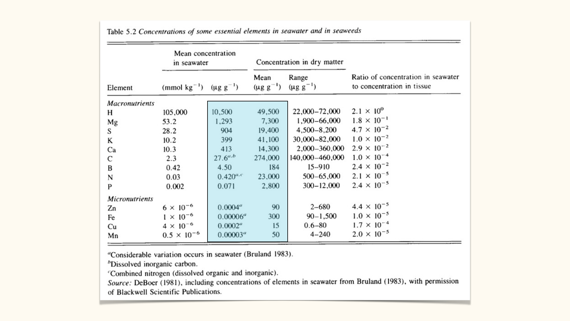
A key physiological contradiction prompts interesting questions: inside the plant, the concentration of key nutrients is typically much higher than outside — in seawater or soil. For example, iron, a particularly scarce element in seawater, is maintained at relatively high tissue concentrations, which demands an energetic uptake strategy (the same applies to most other minerals and nutrients). Passive uptake via diffusion or osmosis cannot account for this, as both processes follow concentration gradients (from areas of high to low concentration).
Therefore, nutrient uptake often requires active transport — energy-dependent mechanisms that move nutrients against their concentration gradient into the plant, where they are assimilated into new biomass.
6 Limiting Nutrients: the Concept and Experiments
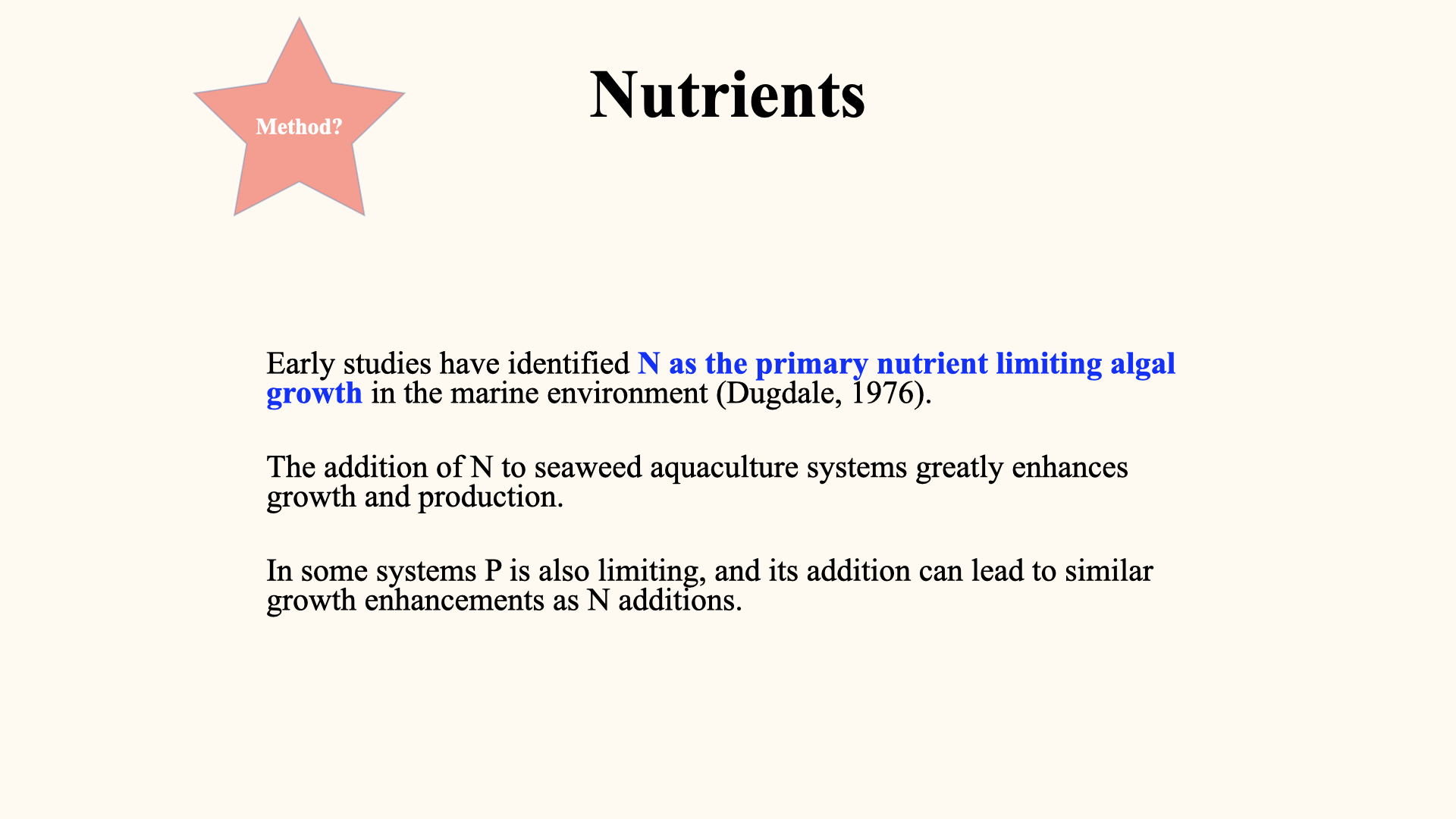
Beginning in the 1960s-70s, researchers recognised that at any time, a particular nutrient could be ‘limiting’. That is, if it is removed or absent, growth ceases. Professor Dugdale and colleagues demonstrated that in most seawaters, nitrogen is the major limiting nutrient. Experiments adding nitrogen to seawater samples resulted in rapid phytoplankton growth; adding other nutrients like phosphorus or potassium generally produced no such effect unless these were limiting.
Therefore, a nutrient is ‘limiting’ in a given context if its addition results in increased growth; if not, it is not currently limiting. In most marine environments, nitrogen is limiting; phosphorus sometimes is, but this is more common in freshwater environments.
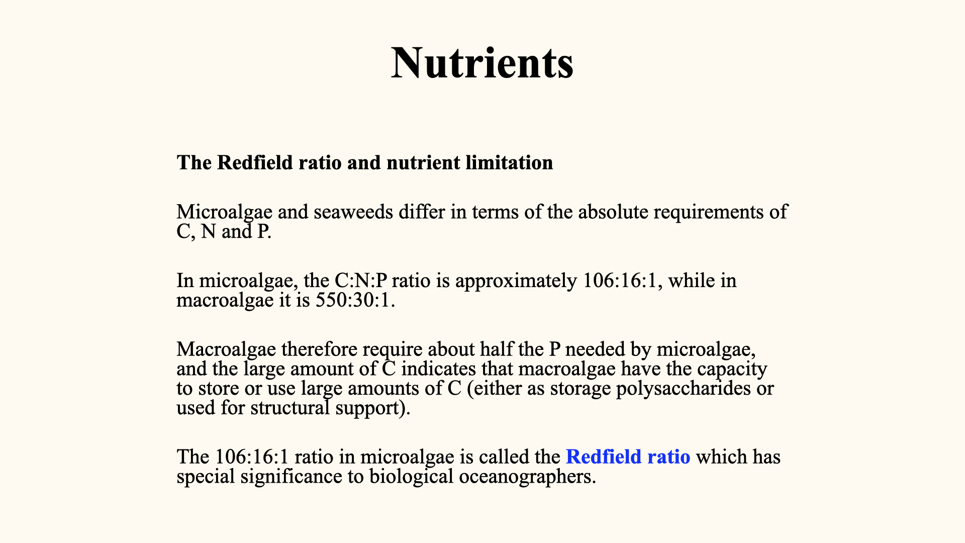
7 The Redfield Ratio and Nutrient Limitation
The “Redfield ratio” is a critical empirical observation: for every \(106\) atoms of carbon in microalgae, there must be \(16\) atoms of nitrogen and \(1\) atom of phosphorus for optimal growth. That is, the ideal \(\mathrm{C}:\mathrm{N}:\mathrm{P}\) ratio is \(106:16:1\).
For macroalgae, a similar ratio exists: \(550:30:1\) (C:N:P), reflecting the greater carbon requirement for structural integrity in larger, multicellular algae.
This optimal ratio is essential. Any deviation means one of the nutrients becomes limiting, restricting growth. Microalgae, being unicellular and minute, need less structural carbon than macroalgae.
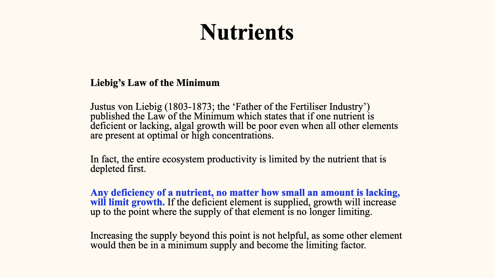
8 Liebig’s Law of the Minimum
Liebig’s law, or “the law of the minimum,” was articulated in the 19th century. It states that the yield of a plant is determined by the single most limiting nutrient, regardless of the abundance of others. Thus, if any one nutrient is below its critical threshold, it will restrict growth, no matter how abundantly everything else is supplied.
This principle is vital for optimising fertilisation strategies in both agriculture and aquaculture: knowing which nutrient is limiting allows for targeted supplementation for maximal growth.
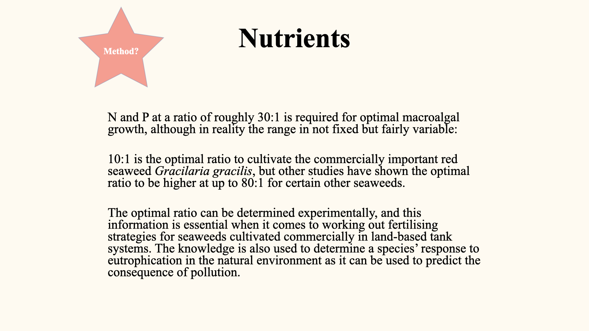
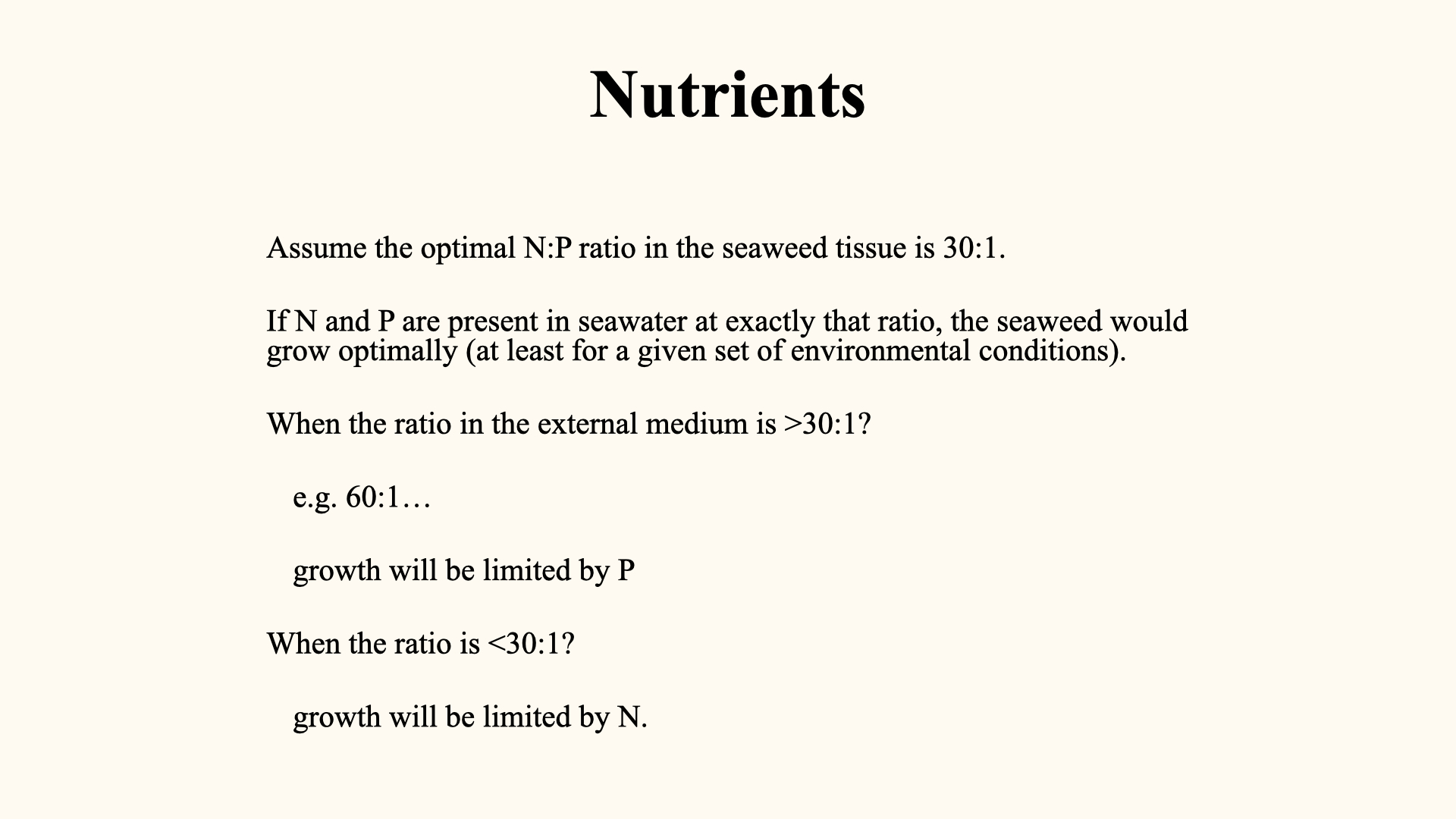
For a red macroalga with an optimal N:P ratio of \(30:1\), suppose more nitrogen is present than phosphorus as required. Phosphorus becomes the limiting nutrient, constraining growth despite surplus nitrogen. Conversely, if nitrogen is below the required ratio, then it is the limiting nutrient.
This concept extends to all primary producers — seaweeds, microalgae, and terrestrial plants.
9 Luxury Consumption
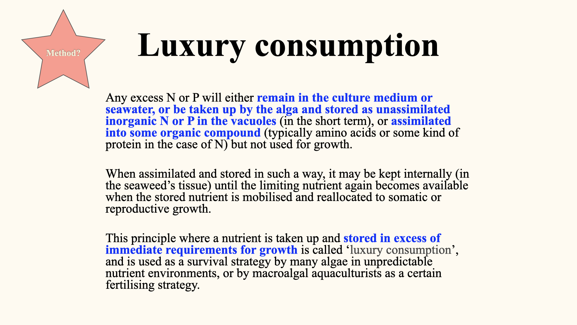
Luxury consumption describes the phenomenon where some plants — particularly certain seaweeds — can take up more of a nutrient than is immediately required for growth, storing the excess for future use. When environmental levels of nitrogen or phosphorus later dip below optimal, the plant draws on these internal reserves to maintain growth.
This adaptation is especially valuable in environments with fluctuating nutrient availability and features prominently in aquaculture. Here, seaweeds can be provided with nitrogen and phosphorus at optimal ratios, and their ability to undertake luxury consumption helps buffer against subsequent scarcity.
Luxury consumption is a survival strategy most evident among K-selected, climax species in the ocean, conferring resilience in the face of unpredictable nutrient supply, and ensuring continued survival and growth despite external variability.
10 Environmental Consequences of Nutrients and Uptake by Seaweeds
Yesterday we spoke about nutrients. I gave you a brief introduction to what nutrients are, and explained that they can be classified into macronutrients and micronutrients, as well as essential and beneficial nutrients. Today, we need to talk about the consequences — the environmental consequences — of nutrients. We will also begin to explore the field of measuring the uptake of nutrients by seaweeds. That is our plan for today.

One of the things we are going to do is to use nitrogen as our example. Nitrogen is convenient and easy to work with. The uptake mechanisms seen in many other nutrients are similar to those for nitrogen, so we can use it as a nice case study. But, of course, nitrogen is also one of the most important nutrients, both in the ocean and on land. It is often a limiting nutrient in the ocean and is important in many environmental problems we face today, such as eutrophication.
This lecture gives the ecophysiological background for eutrophication. We want to understand why some seaweeds respond so rapidly to nutrient enrichment and why certain forms become nuisance algae.
10.1 Case study: the beijing olympics and eutrophication
As an example, I will refer to what happened during the Beijing Olympics in around 2008. Just prior to the Olympics, vast parts of the Chinese shoreline were covered with nuisance green seaweeds. Authorities had to employ a whole group of people to clean up the shoreline. All those green bits — the seaweed blooms in China — were a direct result of nitrogen entering the ocean and polluting the waterways. It is unsightly, it is smelly, and it is dangerous, so it is a huge problem around the world.
10.2 Sources and forms of nitrogen
So, where does nitrogen come from? Nitrogen is quite abundant in the atmosphere — actually, the bulk of the atmosphere is comprised of nitrogen, about 79% of it is gaseous nitrogen, \(N_2\). Gaseous nitrogen itself cannot be used by plants, so certain processes are required to convert that nitrogen into a bioavailable form that plants can take up.
Nitrogen is brought into the oceans via rivers, mostly in the form of nitrate and ammonium. It can also be present in the atmosphere as nitrous oxides and, in water, as nitrous oxides, entering the ocean via river runoff or various atmospheric processes. Other sources include processes in the Earth’s crust, like volcanic eruptions, as well as fossil fuel burning from industrial operations, which both put nitrous oxides into the atmosphere. In certain cases, that nitrogen becomes available as a very acidic form — nitric acid — which is a source of some acid rain.
But once the nitrogen enters the ocean, many interesting processes take place. It gets recycled, taken up by algae, released by algae, released by animals that feed upon the algae — so the whole big global biogeochemical process is seen in the ocean, as well as elsewhere on the planet.
We will return to the larger biogeochemical cycles shortly.
10.3 Nitrogen fixation and cycling
As I said before, gaseous nitrogen in the atmosphere, which is the bulk of it, cannot be used directly by plants. It must somehow become available, and this is accomplished by the process of nitrogen fixation, carried out by organisms such as cyanobacteria. Cyanobacteria can take up atmospheric dinitrogen (\(N_2\)), lock it internally in organic forms or as ammonia. When the cyanobacteria die and decompose or are eaten, that nitrogen is recycled in the form of ammonium or nitrate back into the ocean. Thus, cyanobacteria fix atmospheric nitrogen, making it available to the rest of the ecosystem to be taken up as ammonium or nitrate. This supports much of the planet’s photoautotrophs, on both land and in the ocean.
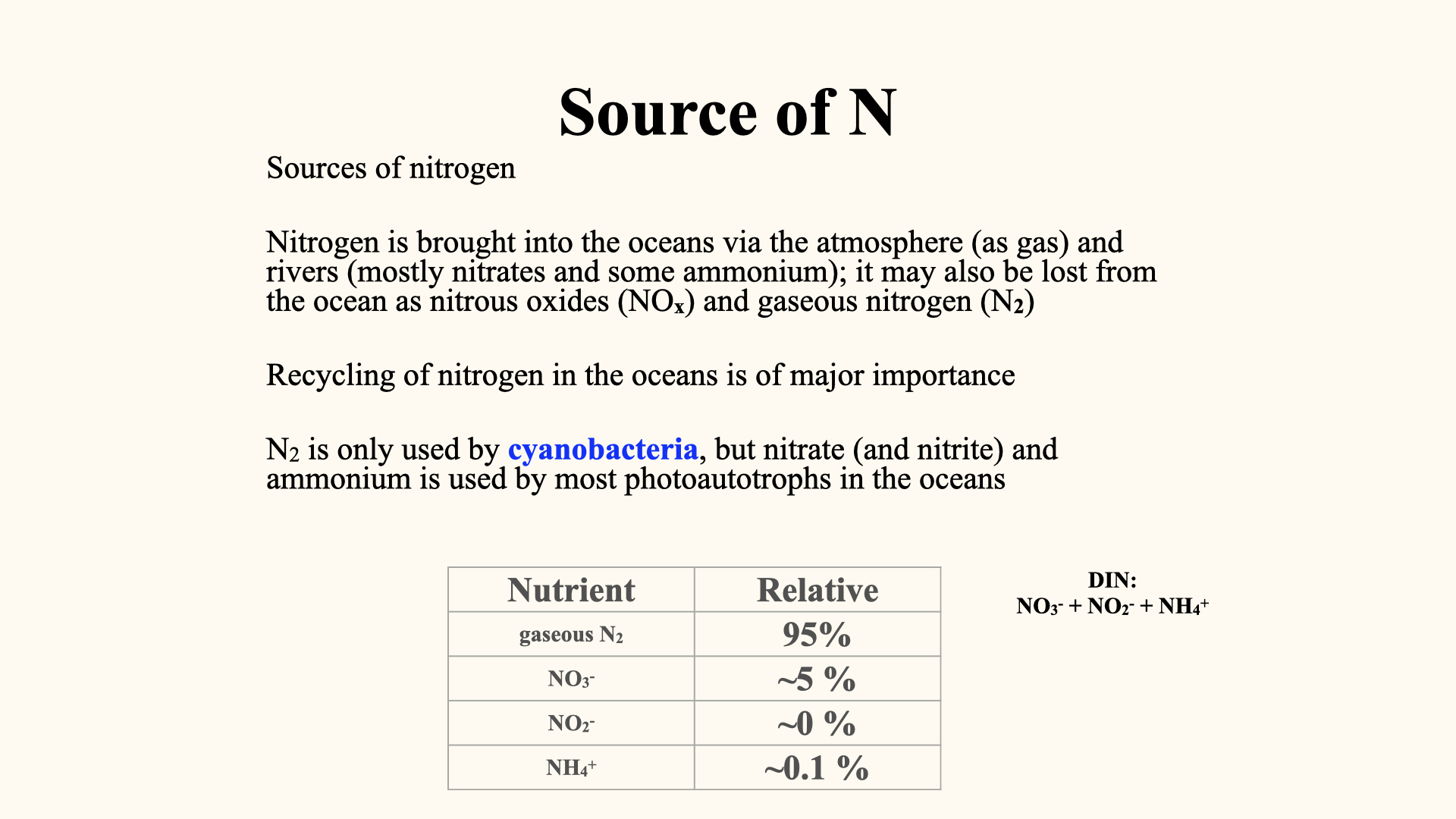
If we look at the various sources of nitrogen: gaseous nitrogen is very abundant in the ocean and atmosphere. In the ocean, once it is dissolved, the total amount of all forms of nitrogen in the ocean is about \(95\%\) or so gaseous nitrogen — meaning dissolved \(N_2\) from the atmosphere. A much smaller fraction is available as nitrate—\(NO_3^-\)—which comprises about \(5\%\) of the nitrogen in the ocean. An even smaller amount is present as nitrite \(NO_2^-\); it is almost immeasurable in many instances, because nitrite is only present in seawater for very short periods as an intermediary between ammonium and nitrate. Concentrations of nitrite are, therefore, very low.
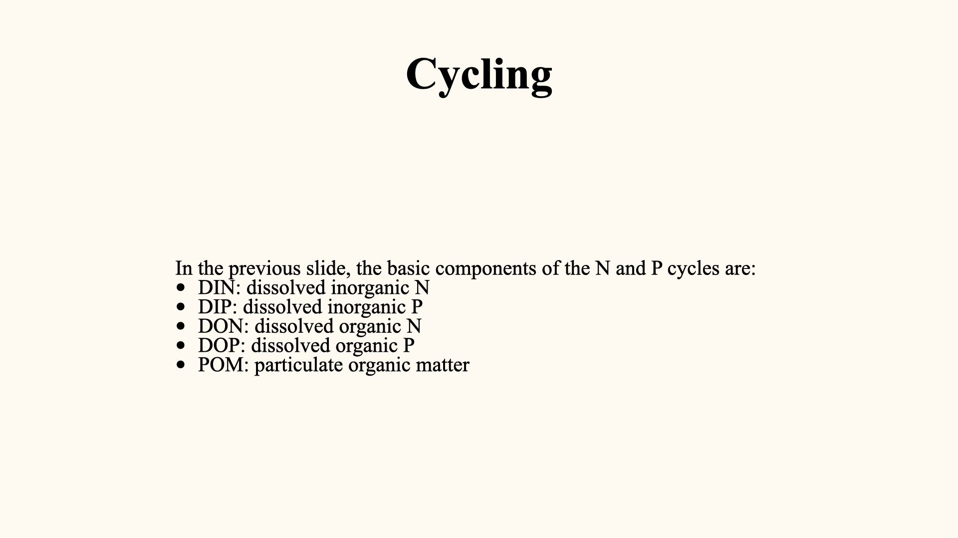
Nitrogen is also present as ammonium (\(NH_4^+\)); close to about \(0.1\%\) of the total nitrogen in the ocean is present as ammonium. So those three compounds—\(NO_3^-\), \(NO_2^-\), and \(NH_4^+\) (nitrate, nitrite, and ammonium)—are together known as DIN: dissolved inorganic nitrogen. This is the amount of nitrogen available for uptake by plants in the ocean.
“Dissolved” because it is in ionic form, within the water; “inorganic” because, while it is not bonded within an organic molecule, it does not contain carbon-hydrogen structures; and “nitrogen” because the major macronutrient atom in all these is nitrogen.
10.4 The marine nitrogen cycle
Once nitrogen enters the ocean, it is cycled in various different ways. It is a complex set of reactions and processes, involving uptake by phytoplankton, their death, their consumption by zooplankton and fish, as well as decomposition — a whole host of processes.
The science that studies the transformation of various forms of nutrients between abiotic and biotic pools within the Earth system is called biogeochemistry. Biogeochemistry is concerned with the movement and the rates of transformation of nutrients between, for example, phytoplankton and zooplankton (organic or biotic components), the ocean (the hydrosphere), the atmosphere, and the geosphere.
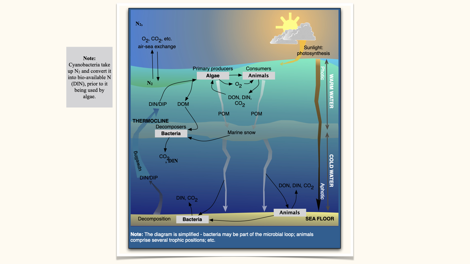
Here is a basic, simplified representation of the nitrogen cycle in the ocean: At the top, you have the atmosphere, at the bottom the ocean floor, and in between is the water column. In and out of the atmosphere, gases such as \(O_2\), \(CO_2\), and \(N_2\) move into the ocean, so we end up with DIN (ammonium, nitrate, nitrite) dissolved in the water. Algae then take up this DIN to produce algal biomass via photosynthesis. Animals consume phytoplankton, relying on them for biomass production, and in turn carry out respiration, taking up oxygen produced by the algae.
As animals eat algae, they excrete waste products, releasing \(CO_2\), more DIN, and dissolved organic forms of nitrogen into the water. In feeding on algae, animals might only consume parts, allowing algal cell contents to leak out, making dissolved organic nitrogen (DON) available to the environment. Algae can then take up this DON.
Here, you see a cycling: nitrogen comes from the atmosphere, dissolves in seawater, is taken up by algae, consumed by animals, and released again. But not all nitrogen is continually cycled — some is lost. Particulate forms of nitrogen, called POM (particulate organic matter), settle down through the water column as “marine snow.” As it falls, marine snow is decomposed by bacteria, which release more DIN and \(CO_2\) in the process. Thus, concentrations of DIN generally increase deeper into the ocean, as marine snow decomposes and releases more nutrients.
10.5 Remineralisation and upwelling
Animals on the seafloor can consume marine snow, releasing DIN, DON, and \(CO_2\) into the water column, with bacteria contributing to remineralisation. Remineralisation is the process that converts organic forms of nitrogen back into inorganic forms like ammonium and nitrate.
Over time, DIN accumulates in the deeper ocean, but physical ocean processes, such as ocean currents (upwelling), transport some of this deep, nutrient-rich water back to the surface, injecting remineralised nitrogen into sunlit upper layers, where algae can again take it up.
So, these cycles are coupled by biological processes — linking algae to animals through heterotrophy (predation, grazing), decomposition, excretion, faecal pellet production, as well as by physical processes like upwelling. Photosynthesis is a surface process, so nitrogen uptake by algae occurs mainly in surface waters, not in the deep ocean where there is no light.
Also, do not forget the role of nitrogen-fixing bacteria like cyanobacteria, which fix atmospheric nitrogen and make it bioavailable for oceanic and other organisms. This is how atmospheric nitrogen becomes available in the surface ocean.
10.6 Definitions: some key terms
Some important definitions:
- DIN: Dissolved Inorganic Nitrogen; includes ammonium, nitrate, nitrite.
- DIP: Dissolved Inorganic Phosphorus; phosphorus equivalents to DIN.
- DON: Dissolved Organic Nitrogen.
- POM: Particulate Organic Matter; also includes particulate forms of both nitrogen and phosphorus.
The biogeochemical cycle operates similarly on land, but most of the transformations happen within the soil, particularly around plant roots, as well as via aboveground decomposition processes — for example, as leaves fall, decompose, and transfer nitrogen back into the soil.
10.7 Units, concentrations, and oceanographic patterns
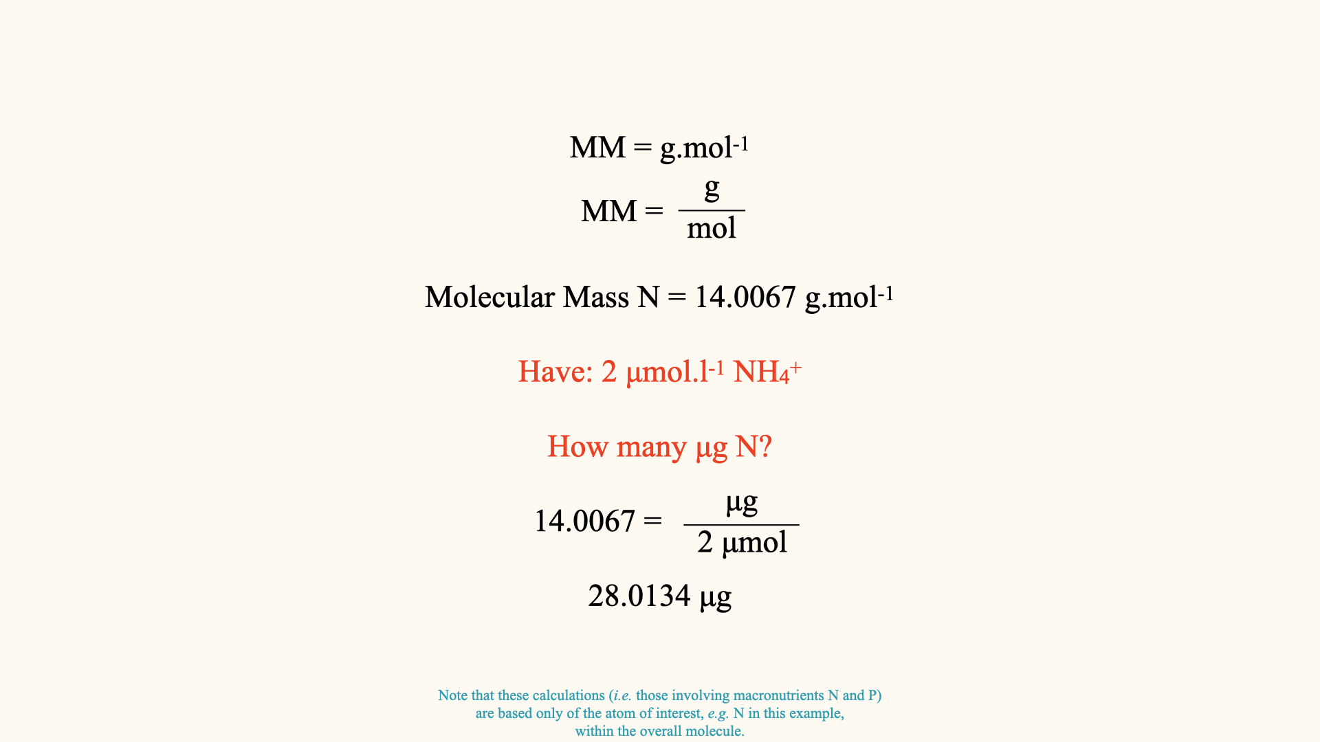
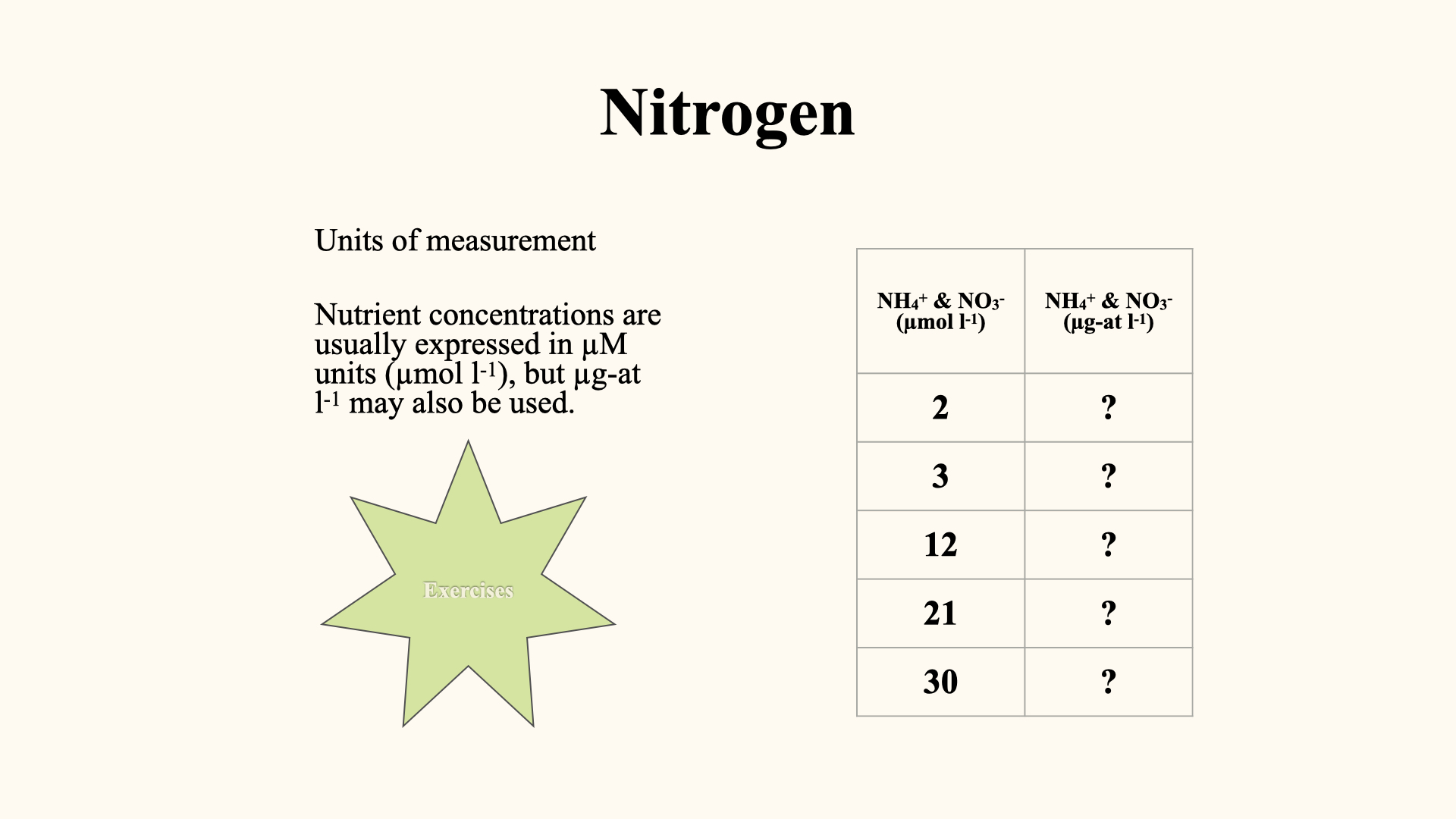
When reading literature about nitrogen as a macronutrient, you will encounter various units: micromolar (\(\mu\)M), microgram atom per litre, and so on. These all describe the concentration of nitrogen in water or solid solution. You should recall from first-year chemistry how to convert between micromolar and microgram atom per litre (\(\mu\)M to \(\mu\)g atom L\(^{-1}\)), and vice versa. Be familiar with these conversions, as you will encounter them in tests.
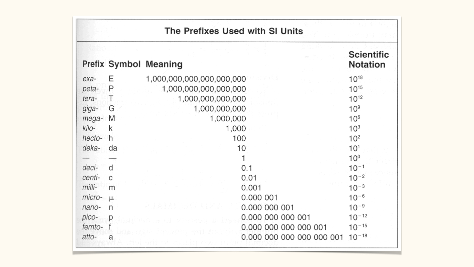
You must also know the SI prefixes and the number of zeros associated with each — grammes, milligrammes, microgrammes, nanogrammes, picogrammes, et cetera. In plant physiology, a basic grasp of chemistry and SI unit prefixes is assumed.
10.8 Typical oceanic nitrogen concentrations
Here is a range of concentrations that nitrogen is available in the ocean:
- Tropical regions (ca. \(10^\circ\)S to \(10^\circ\)N): Very low nitrogen; concentrations may be in the nano- to picogramme range (\(\mathrm{ng\ L^{-1}}\) — \(\mathrm{pg\ L^{-1}}\)).
- Most of the ocean: Microgramme to milligramme range.
- Freshwater systems: Often reach the milligramme range.
- Upwelling regions (e.g., the Benguela upwelling off South Africa, Canary Current off North Africa, Humboldt off South America, California Current off North America): Highest oceanic nutrient levels. Here, total inorganic nitrogen can reach up to \(40\ \mu\mathrm{mol\ L^{-1}}\), while inorganic phosphorus typically reaches \(2\ \mu\mathrm{mol\ L^{-1}}\).
Note the ratio here, approximately 10:1, closely corresponding to the Redfield ratio.
During active upwelling, nutrient concentrations rise to \(20\)–\(40\ \mu\mathrm{mol\ L^{-1}}\) nitrogen, \(2\ \mu\mathrm{mol\ L^{-1}}\) inorganic phosphorus. When upwelling subsides, these values drop below \(4\ \mu\mathrm{mol\ L^{-1}}\) for nitrate and \(0.2\ \mu\mathrm{mol\ L^{-1}}\) for inorganic phosphorus.
Thus, in the ocean, background nitrogen levels are not fixed but fluctuate, sometimes very rapidly (over tens of minutes) due to oceanographic processes such as upwelling. Algae have evolved various adaptations to cope with the intermittent and transient nature of nitrogen availability in the ocean — a stark contrast to terrestrial systems, where changes are usually slower.
10.9 Classification of oceanic systems based on nutrient levels
The ocean can be classified into:
- Oligotrophic: Low nutrient, e.g., tropical regions, almost no nitrogen.
- Mesotrophic: Intermediate, e.g., upwelling zones, fluctuates temporally.
- Eutrophic: High nutrients, often due to human influence — unnaturally high nitrogen.
In the ocean, nitrogen is typically limiting. However, excessive input causes problems — most notably, eutrophication.
10.10 The nitrogen bomb: human impact
For your self-study: read the article “The Nitrogen Bomb” (available on Ecoma). The Haber-Bosch process has resulted in a huge problem worldwide in both terrestrial and aquatic systems. “Nitrogen bomb” is a metaphor for the disastrous potential of excessive and unwisely applied nitrogen, most sharply observed in eutrophication. This is examinable content.
10.11 What is eutrophication?
Eutrophication usually occurs when too much nitrogen is added to a body of water that would naturally be nitrogen limited. In these systems, certain algae or seaweeds respond rapidly to the enrichment. For instance, the three illustrated species all possess high surface area to volume ratios, meaning nearly every cell is exposed directly to the environment and can immediately take up available nutrients. This capacity allows rapid growth and biomass accumulation.
More complex seaweeds with lower surface area to volume ratios respond more slowly, if at all, to such nutrient pulses; the response is more distributed and structurally limited. In contrast, these high surface area opportunistic algae (sometimes called R-selected species) bloom excessively when nutrients are introduced, becoming nuisance species and disrupting the ecological balance.
In a natural system, there is a high diversity of plants and animals. After eutrophication, one species becomes dominant, reducing community composition, species richness, and causing the biomass of that one species to increase exponentially.
In severe cases, the system can become anoxic. Imagine a dense bloom of photosynthesising algae; at night, without photosynthesis, respiration consumes all the oxygen in the water. Species that require oxygen die off, and their decomposition consumes even more oxygen, eventually producing low-oxygen, or dystrophic, conditions.
Bacteria are key to these processes, as they drive decomposition and thus increase total ecosystem respiration and oxygen consumption.
10.12 Mitigating eutrophication
As for what can be done: removing the blooming nuisance algae is not addressing the underlying issue. We must ensure that sources of nitrogen entering the water are addressed — by improving sewage treatment, reducing fertiliser runoff from agriculture, and proper waste management. Rivers seen as convenient dumping grounds simply transfer the problem downstream; the consequences are borne by someone else or by the ecosystem.
11 Linking Form and Function: Surface Area to Volume Ratio
I have mentioned that response to eutrophication is connected to both the morphology and physiology of algae. Those species with high surface area to volume ratios can absorb nutrients rapidly and outcompete others. This is where Littler and Littler’s “functional form model” comes into play, explaining why morphology is crucial to ecological dynamics under eutrophic conditions.
At this point you should connect two ideas that now belong together in this module: surface area to volume ratio and nutrient uptake. High-SA:V forms can capture nutrient pulses rapidly, which is one reason eutrophication often shifts communities toward opportunistic algae.
If you have questions or do not grasp a particular aspect, you are welcome to ask on WhatsApp. Please ensure you read the assigned articles and refresh your knowledge of unit conversions and SI prefixes, as you will be expected to use this knowledge fluently.
Read further on eutrophication. Much more can be said, but the core is straightforward biology playing out in an ecosystem that simplifies under stress — one species dominates as nutrients increase, reducing diversity and altering physiological and ecological processes within the system.
12 Nutrient Uptake
Today, I want to discuss the physiology of plant nutrient uptake, specifically focussing on the processes by which algae — seaweeds, in marine environments — take up nutrients from their surroundings. Throughout this lecture, I will be using the terms ‘algae’, ‘seaweed’, and ‘plant’ interchangeably; for the purposes of our discussion, they all refer to seaweeds, as the experiments we are considering were conducted with seaweeds. The uptake processes in terrestrial plant roots are similar regarding the mechanism of transfer from the environment into the plant, but the main differences lie in the environmental processes within soils.
Our goal is to develop an ecophysiological understanding of how plants (seaweeds) absorb nutrients, which will also help explain how seaweeds thrive in various marine habitats, and why many can become nuisance species under eutrophic conditions.
12.1 Pathways and barriers to nutrient uptake
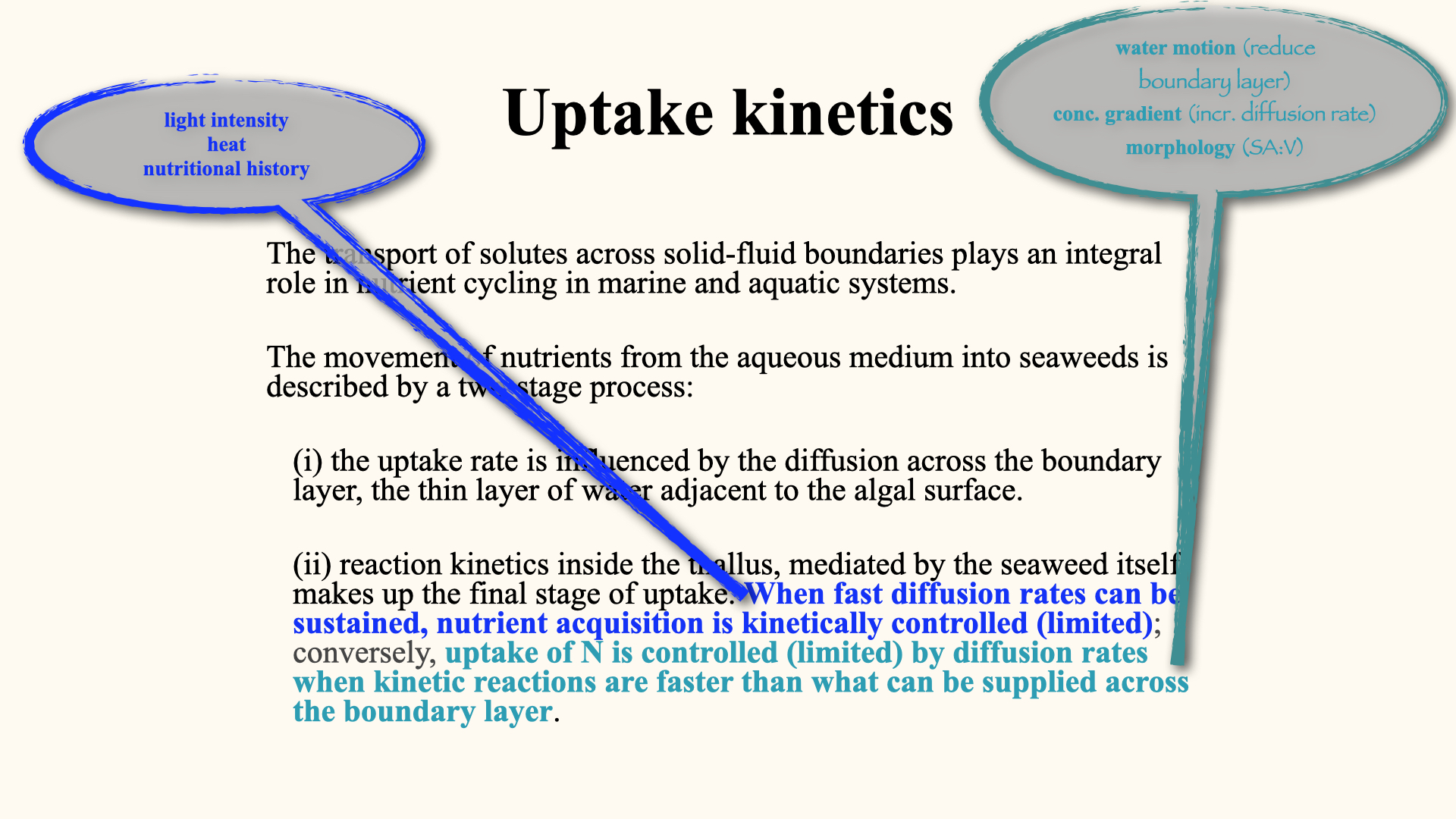
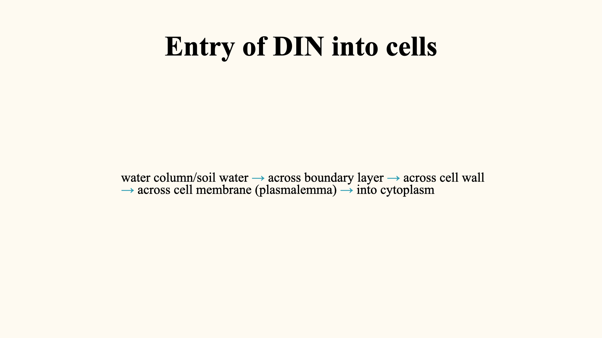
When nitrogen or any other nutrient is taken up, its pathway runs from the water column (or surrounding soil water), across a thin, static barrier of still water adjacent to the cell wall or membrane, known as the boundary layer. From there, nutrients cross the cell wall and membrane, entering the cytoplasm. The uptake of solutes across these solid-fluid boundaries is a key process in nutrient cycling across aquatic, marine, and terrestrial ecosystems.
Nutrient uptake can be described as a two-stage process:
External Phase: Processes taking place outside the plant cell, primarily governed by the diffusion of nutrients across the boundary layer. This thin, unmoving water layer is held close to the algal surface by hydrostatic and intermolecular forces.
Internal Phase: Once nutrients have crossed the membrane, internal processes — especially enzymatic reactions — rapidly convert inorganic nutrients into organic forms. Enzymatic reaction rates, described as reaction kinetics, control how swiftly nutrients such as ammonium or nitrate are metabolised into amino acids, proteins, and other cell constituents.
When assessing nutrient uptake, it is important to distinguish between these two phases. If diffusion from the environment is very rapid, then the overall rate is limited by how quickly the plant’s enzymes can process the nutrients — in other words, the internal, kinetically controlled processes. Not all plants possess the same enzymatic processing rates; some transform nutrients quickly, others more slowly.
Conversely, if environmental diffusion is slow, the uptake rate is limited by external physical processes, rather than by the plant’s internal processing capacity.
12.2 Factors influencing nitrogen uptake
Nitrogen (and other macronutrient) uptake is influenced by many factors:
- External Conditions: The thickness of the boundary layer and the actual concentration of nutrients in the water are crucial. These are influenced by physical conditions outside the plant.
- Form of Nutrient: Ammonium is taken up much faster than nitrate; nitrate requires active uptake, while ammonium is acquired via passive diffusion.
- Nutrient Starvation History: Plants recently starved of nutrients will uptake rapidly when exposed to fresh supply; non-starved plants may not show a significant response.
- Environmental Conditions: High light intensity and high temperatures both enhance metabolism and, consequently, increase \(V_{max}\), speeding up uptake rates.
- Surface Area to Volume Ratio: As discussed, this has a substantial effect on uptake dynamics.
- Mechanisms of Uptake: The presence of additional mechanisms (such as facilitated diffusion) can also influence overall nutrient uptake.
All of these together influence the rate at which macronutrients such as nitrogen and phosphorus are taken up from the environment.
12.3 The boundary layer concept
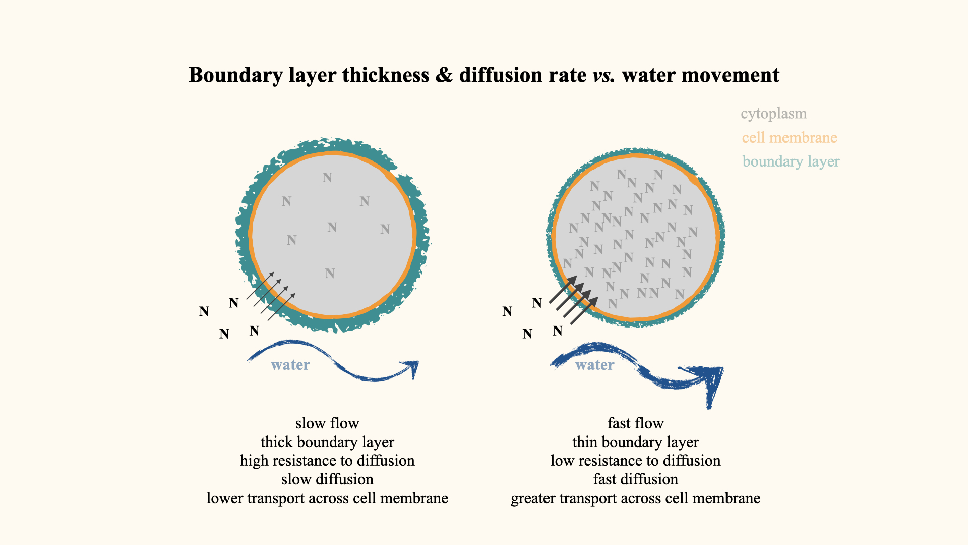
Let me illustrate the boundary layer effect. Picture a plant cell in still water: the cell membrane (orange in our diagram) is surrounded by the boundary layer — a static skin of water held onto the surface. The thickness of this layer is influenced by water movement: in still conditions, it is thick; with greater water motion, it becomes thinner.
The boundary layer acts as a resistance barrier to diffusion. The thicker it is, the greater the distance and resistance for molecules diffusing from the environment into the cell, thus lowering the flux (rate) of nutrient transfer. Where water moves rapidly, the boundary layer thins, reducing resistance and allowing greater nutrient movement into the cell.
Thus, in turbulent waters, plants take up nutrients more efficiently; in still waters, uptake is limited due to the thick boundary layer.
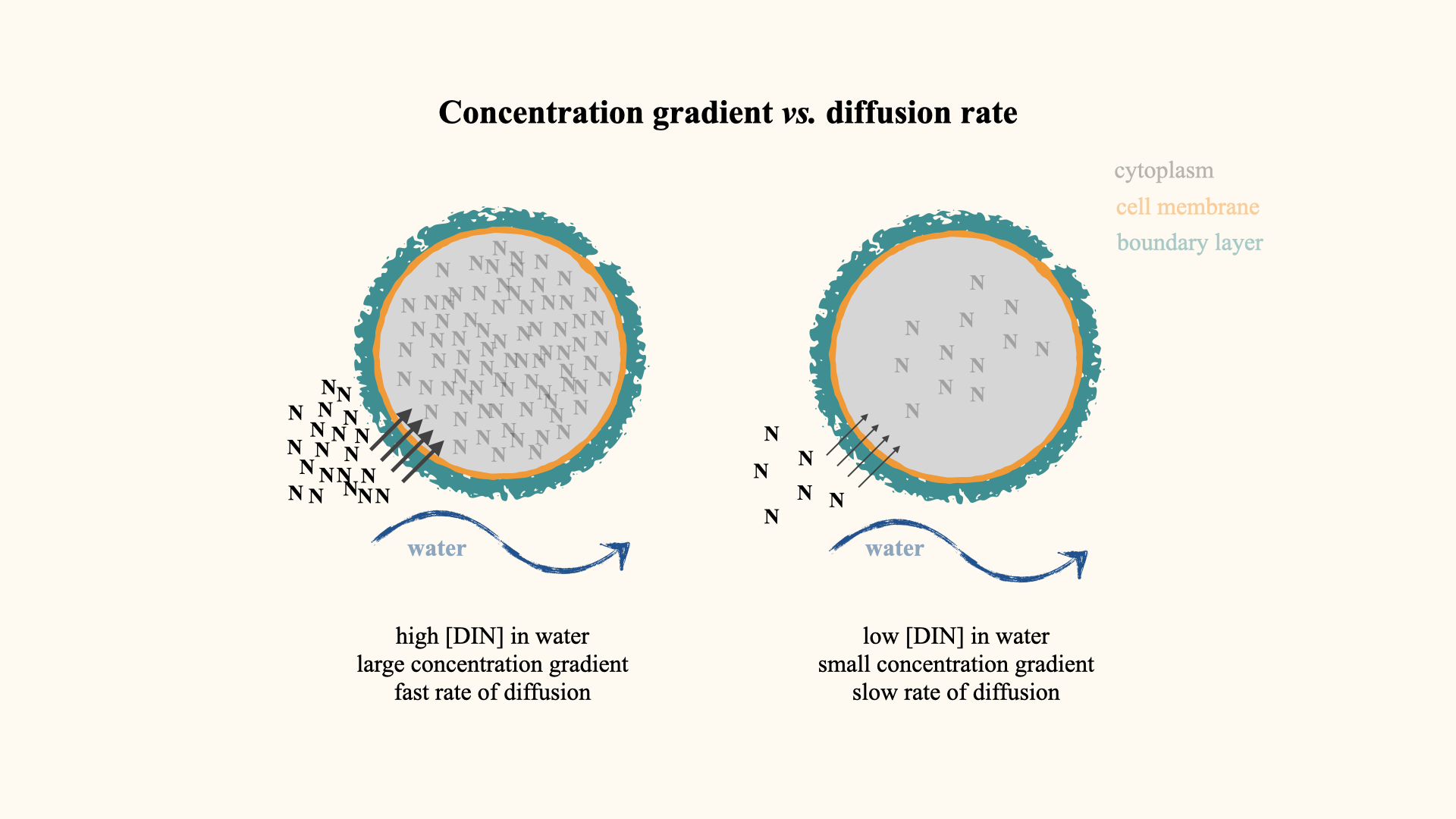
12.4 Influence of environmental nutrient concentration
Water movement is not the only factor affecting uptake. Another is ambient nutrient concentration. With identical water movement, a cell surrounded by a high nutrient concentration will experience a steeper concentration gradient, promoting greater nutrient flux into the cell. The rate of diffusion is directly proportional to the gradient between external and internal nutrient levels.
In very low-flow conditions, increasing the concentration of external nutrients can compensate somewhat for a thick boundary layer, enhancing uptake despite slow water movement.
These two principles — the thickness of the boundary layer (and thus water movement) and the nutrient concentration gradient — underlie the role of the diffusion step in limiting nutrient uptake.
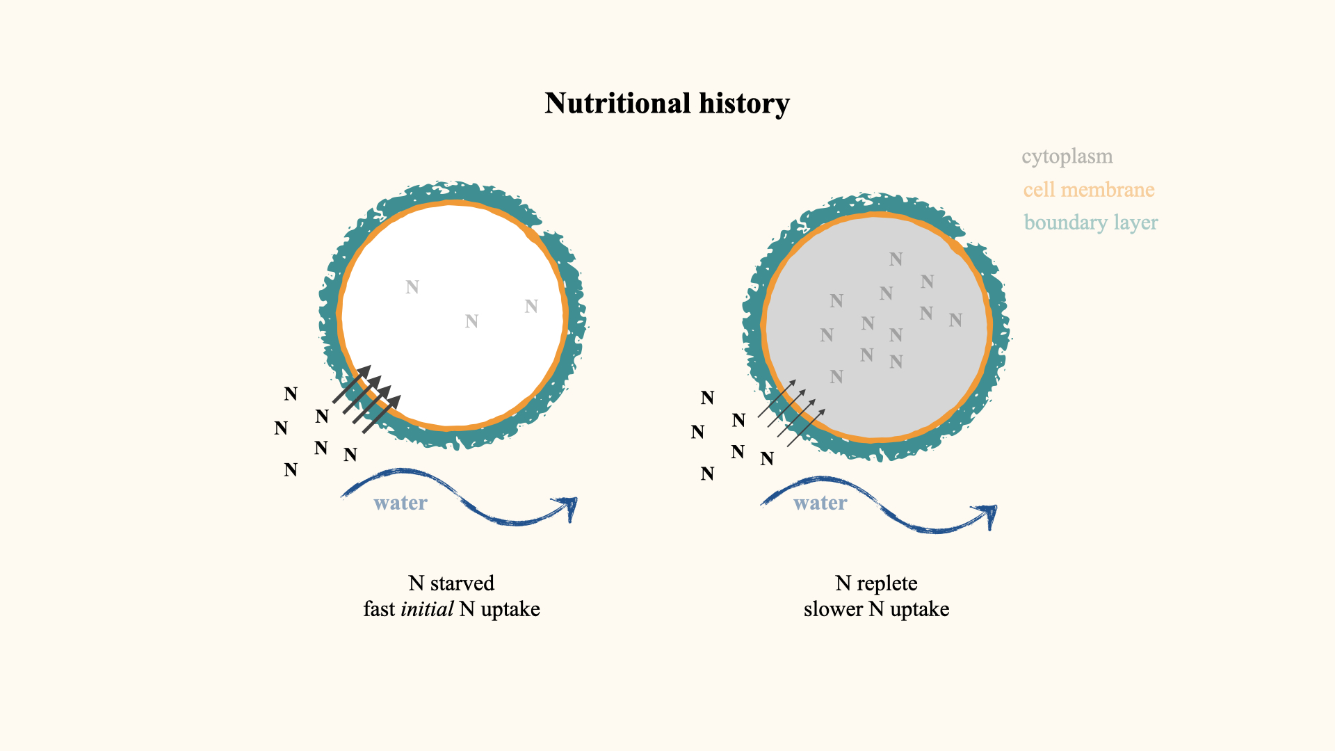
12.5 Algal nutritional history
Another way in which nutrient uptake is affected — this time due to properties within the interior of the plant cell or algal cell — is when you have algae that have been starved of nutrients for an extended period. For instance, in situations in the ocean characterised by periods of low nutrient availability, such as during the non-upwelling phases (downwelling) in upwelling systems, the continued growth of algae, despite the limited external supply, results in diminished concentrations of internal nutrients within the algal cells.
Consequently, when these nutrient-depleted, or nutrient-starved, cells are subsequently transferred into seawater with a high concentration of nutrients, the rate of nutrient uptake increases dramatically. If you then compare the nutrient uptake rate of these nutrient-starved cells to seaweed or algal cells that have a history of recent exposure to nutrients — in other words, where the internal nutrient concentration is much higher — you will find a marked difference. Specifically, if you compare the rate of uptake between nitrogen-starved algae and nitrogen-replete algae, the uptake rate in the starved cells will be far greater than in the nitrogen-replete cells. The reason for why this big difference exists will become clearer later on.
13 Measuring Nutrient Uptake in the Laboratory
A highly detailed protocol for conducting nutrient uptake experiments is provided in “Lecture 8b: Uptake Kinetics — Michaelis-Menten.”
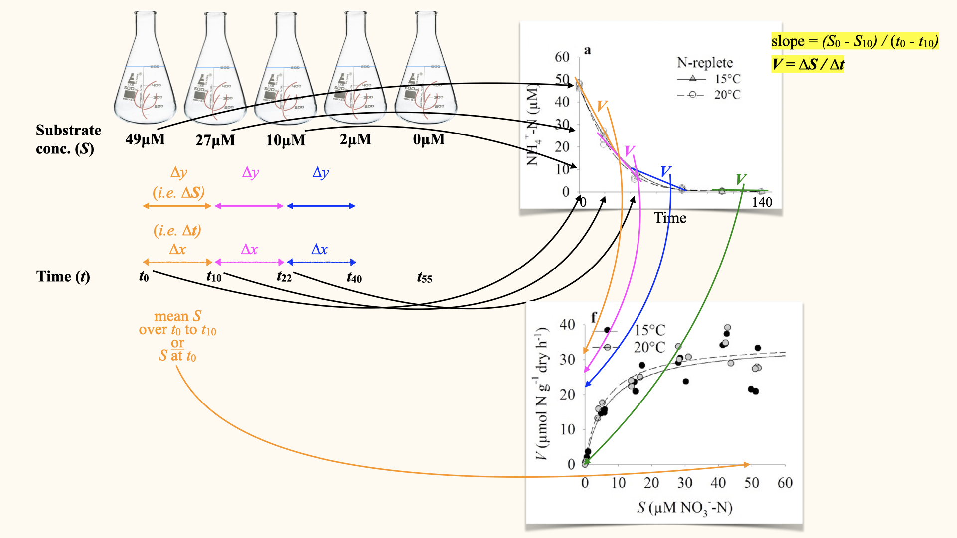
To quantify nutrient uptake in plants, algae, and seaweeds, we perform controlled experiments in laboratory flasks. Here is the protocol I followed for my PhD research:
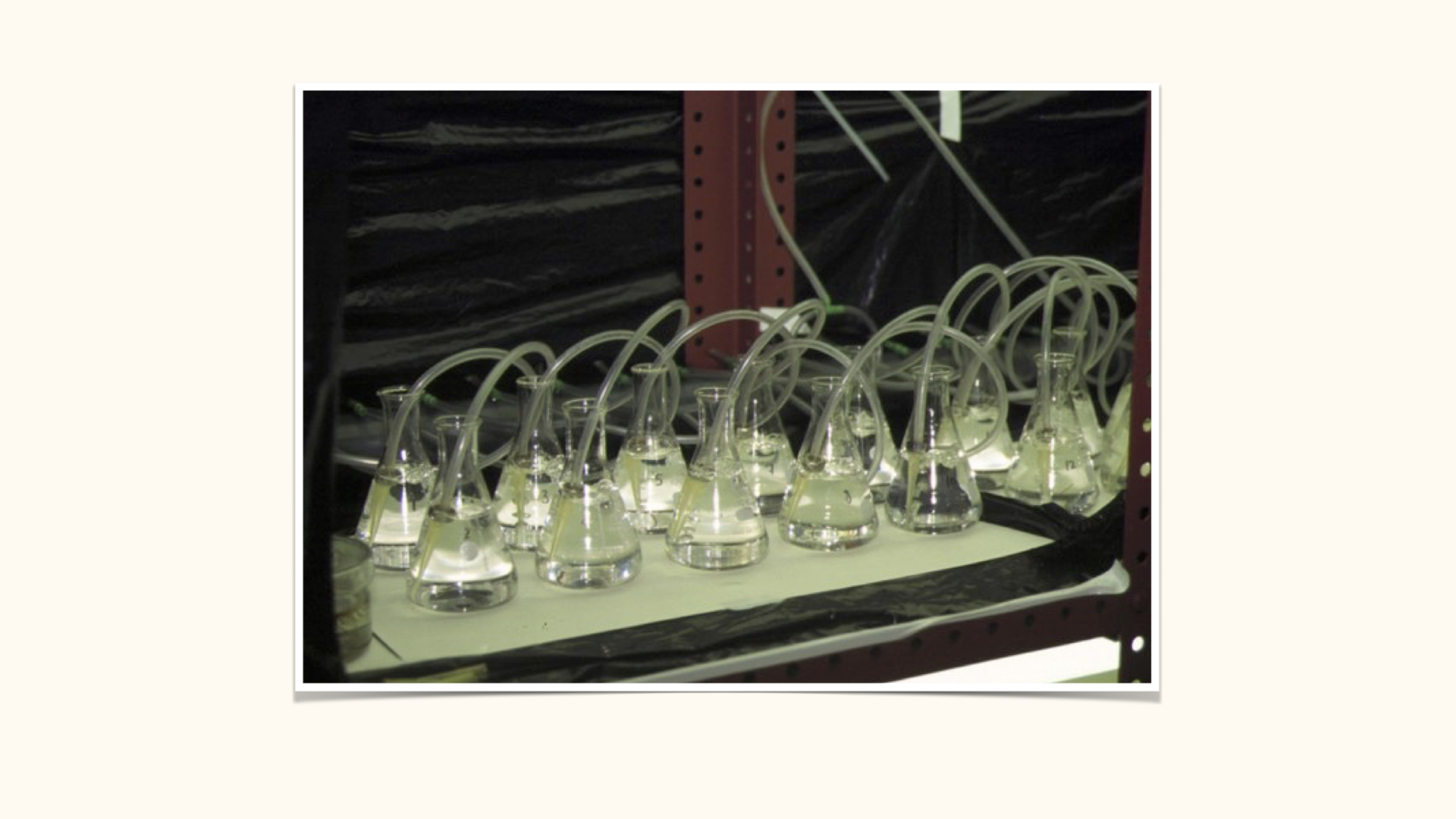
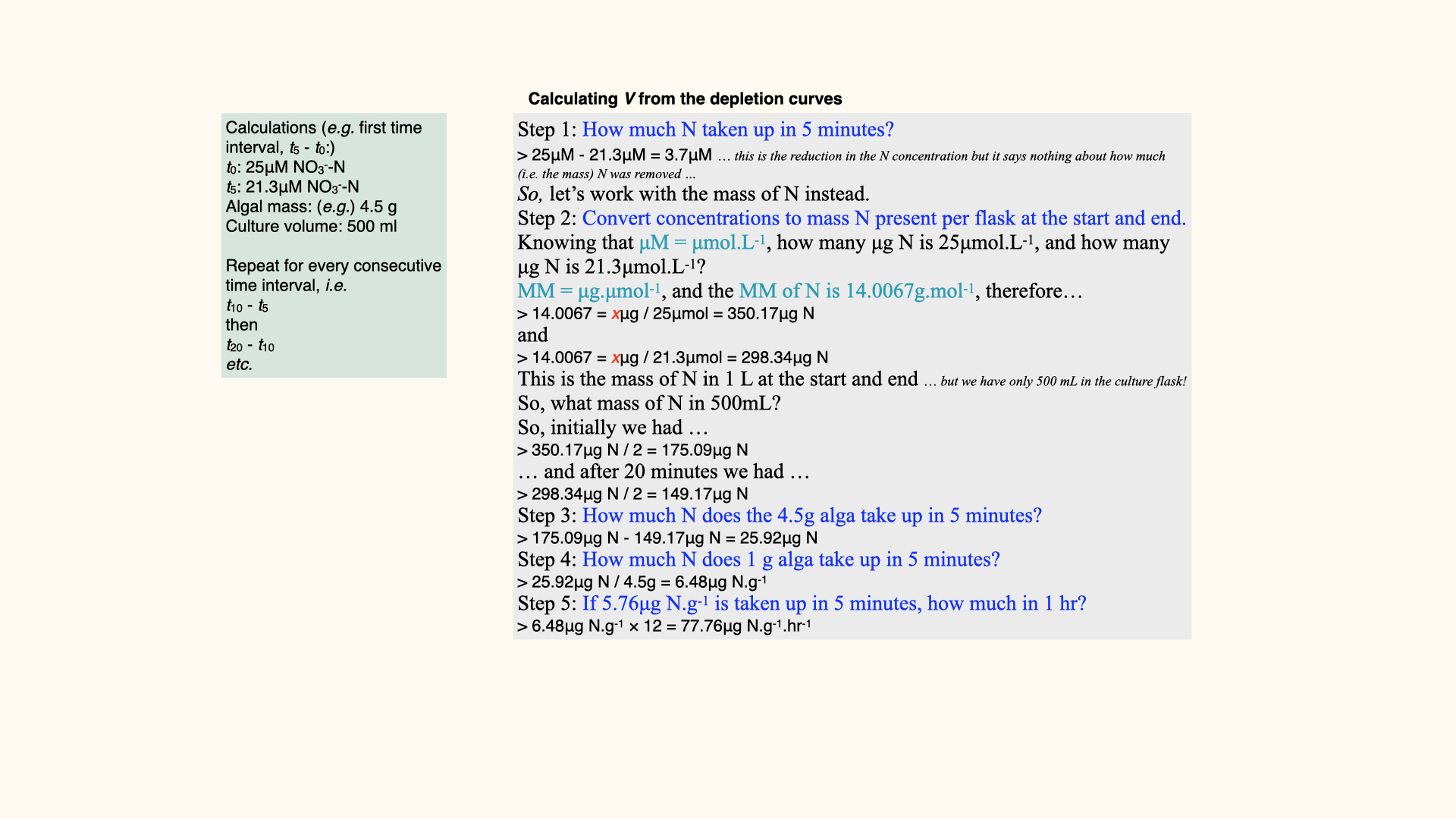
Each flask contains seawater with a known, enriched nutrient concentration and a measured piece of seaweed. At both the start and end of a timed interval (usually 20 minutes), water samples are taken to measure nutrient concentration. The decrease in nutrients reflects uptake by the seaweed.
We also introduce bubbling into the flasks to facilitate water movement, thereby thinning the boundary layer and promoting diffusion. Without bubbling, the boundary layer thickens, reducing nutrient uptake.
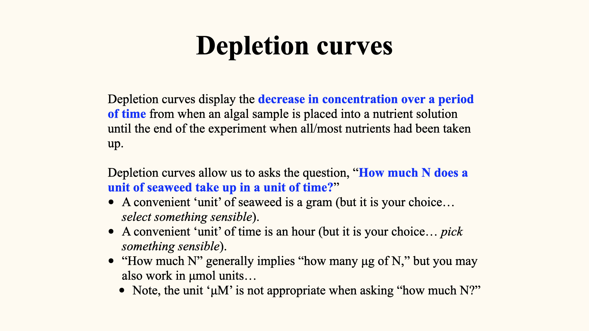
Something that we need to keep in mind when we design these uptake experiments, and when we calculate depletion curves, is that we need to be very certain of the units of measurement that we use during the conduction of our experiment. Typically, we would want to select a certain amount of seaweed — the mass of seaweed that we are going to place within a certain volume of water — and we are going to measure the rate of disappearance of that nutrient from that water over a certain amount of time. We also have to have an idea of the amount of nutrients present in the water.
Firstly, when we work with seaweeds, a typical mass unit of measurement would be grams. Most of the seaweeds that we can work with are of a size where we can weigh them and represent their mass in a couple of grams to tens of grams. Some of the larger seaweeds would weigh in the order of kilograms, and so on. So, we need to be sure that we use a unit of measurement that is appropriate for the thing being studied.
Nutrient uptake as a process can happen very quickly. It can happen over the space of minutes. Certainly, within a period of less than an hour, we can very easily measure the rate of disappearance of nutrients from the culture medium. So, a convenient unit for time measurement would be per hour. But again, depending on the organism that you are going to study, you will have to pick something sensible and relevant to that organism.
When we talk about the volume of the culture medium (usually dictated by the size of our experimental containers), typically we are going to take a small piece of seaweed, algal tissue excised from the whole plant, and put it into a smaller volume of water. That volume of water is often something that can very easily fit into a flask. So, the units of measurement there would be in the millilitre range. Often, the amount of seawater contained in this experiment is, say, less than a litre. In my experiments, it was \(250\;\mathrm{mL}\) or so, if I remember correctly.
Then, concentration units. There are different ways that we can represent chemical concentrations — that is, the concentration of the nutrient in question. We can measure concentrations in micromolar, for example \(\,\mu\mathrm{mol\,L}^{-1}\) (\(\,\mu\mathrm{M}\)), or we can represent concentrations in micrograms per litre, \(\,\mu\mathrm{g\,L}^{-1}\). Again, be sensible in terms of what unit you choose to represent your measurements in.
It is very important that we know these units right at the beginning of our experiments, because they are going to carry through multiple stages of calculations, so that we represent an uptake rate in a sensible unit such as for moles of nutrients taken up per gram of seaweed per hour, i.e., \(\,\mathrm{mol}\;\mathrm{g}^{-1}\;\mathrm{h}^{-1}\). For example, we normalise data to a ‘unit’ of seaweed — typically, per gram, since different flasks might contain slightly different masses (e.g., \(1.2\,\mathrm{g}\) versus \(1.1\,\mathrm{g}\)). By dividing the uptake rate by available mass, we standardise uptake on a per-gram basis. Similarly, we standardise to unit of time by converting measurements taken over 20 minutes to an hourly rate by simple multiplication. Remember, from past lectures, conversion between units (micrograms and micromolar, for instance) is sometimes required.
13.1 Types of uptake experiments
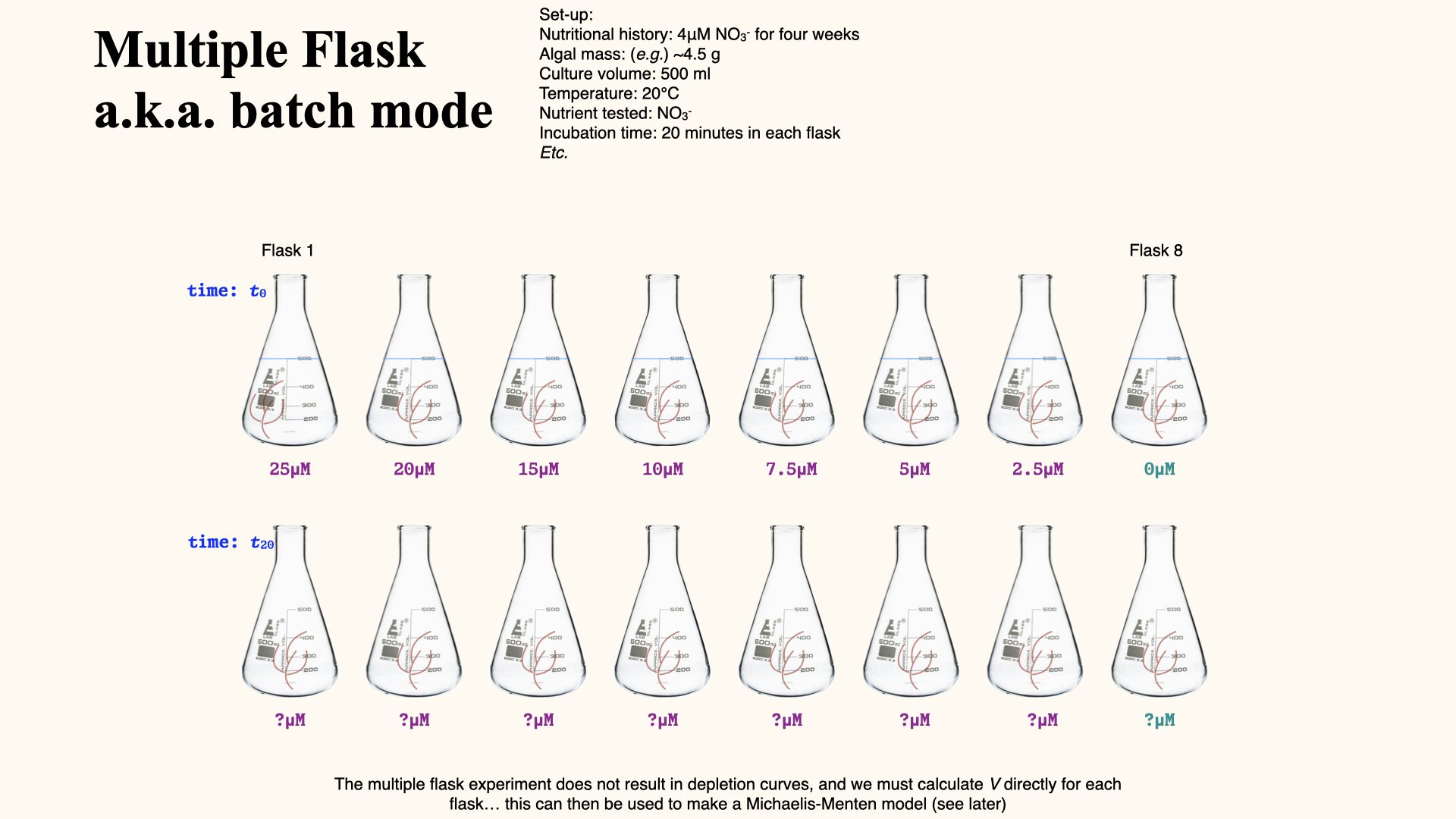
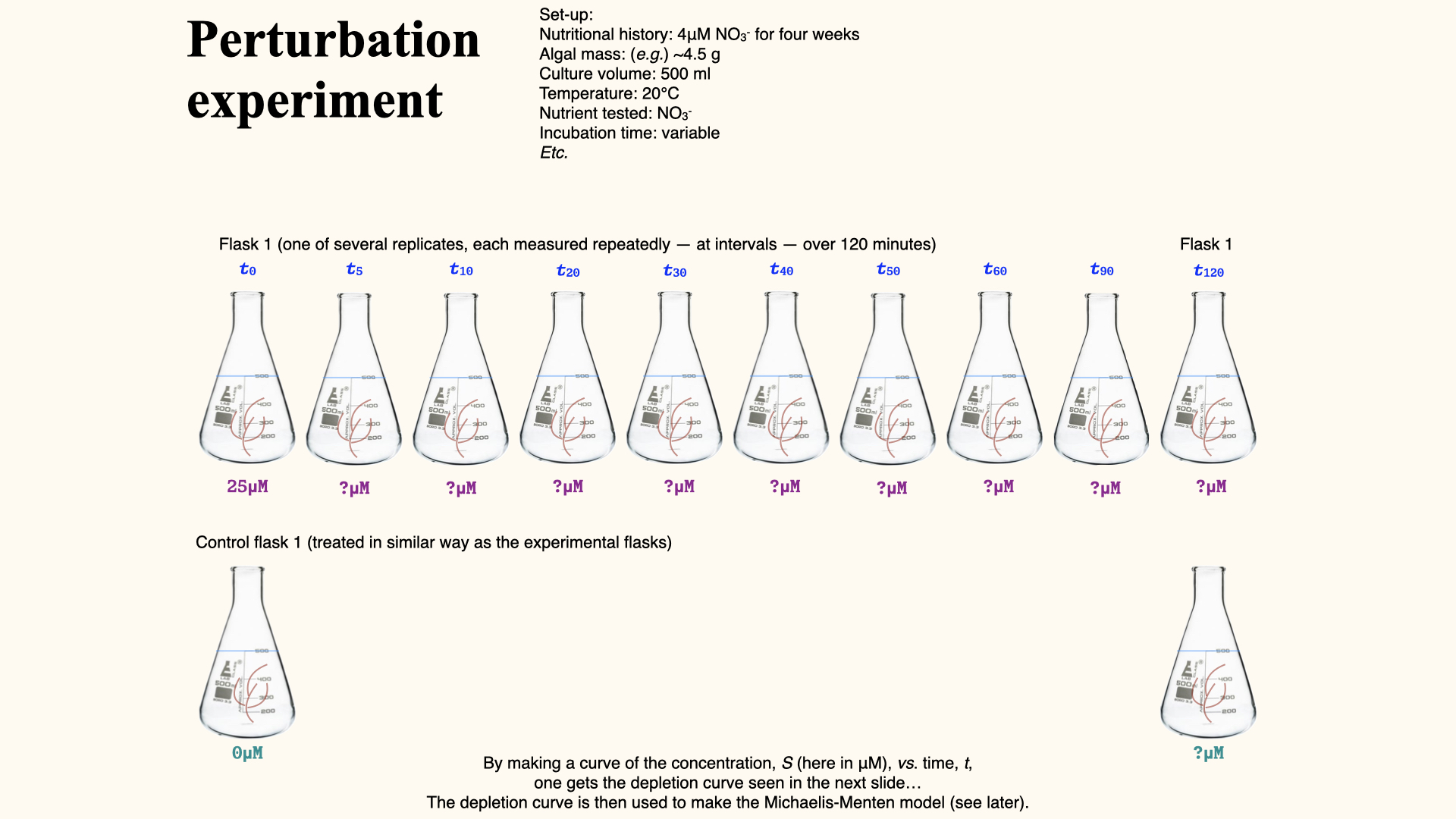
Multiple flask experiment
In a multiple flask experiment, each flask begins with a different initial concentration of nutrient (e.g., \(25\,\mu\mathrm{mol}\,\mathrm{L}^{-1}\), \(20\,\mu\mathrm{mol}\,\mathrm{L}^{-1}\), \(15\,\mu\mathrm{mol}\,\mathrm{L}^{-1}\), etc.), the same amount of seaweed, same water volume (e.g., \(500\,\mathrm{mL}\)), and the same temperature (e.g., \(20^\circ\mathrm{C}\)). After a set duration, changes in nutrient concentration indicate how much has been taken up. Calculations are carefully outlined for you and involve correcting for flask volume, time, and seaweed mass.
You will notice in the figure above that we have a range of concentrations going all the way from about \(25\;\mu\mathrm{M}\) down to \(25\;\mu\mathrm{M}\) concentrations. Why is it that we have \(0\;\mu\mathrm{M}\)? Obviously, no nutrients can be taken up when we have no nutrients present. So, the answer to that question is fairly straightforward: it is a control.
A control is always necessary in our experiment to establish that the only process influencing the mechanism we are studying is the subject of the study — in this case, the nutrients themselves. Therefore, in the \(0\;\mu\mathrm{M}\) flask, what we would expect to observe after \(20\;\mathrm{min}\)—when we remeasure the amount of remaining nutrients in the solution — is that it is still going to be \(0\;\mu\mathrm{M}\).
There are some processes that occur in seawater that can put nutrients back into the water. By having a flask set at \(0\;\mu\mathrm{M}\) nitrogen, we can verify that none of those processes are present within our experiment. In other words, we are controlling for any process that may reintroduce nutrients into the water. If we discover that there is a process that does put nutrients back into the water, we can determine the magnitude of this effect and subtract that from the values we establish for each of the experimental conditions in which nutrients are actually present.
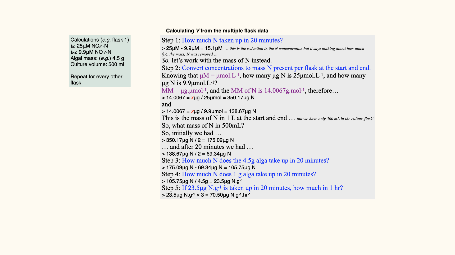
Calculating N uptake in multiple flask experiments
The process of calculating nutrient uptake rates from the depletion curves, which we can establish from the multiple flask experiments, might at first appear complicated. There are indeed many steps involved and multiple points along the way where it is necessary to translate units from one form to another. However, if you understand the process thoroughly, all of these steps become extremely logical and systematic.
It becomes quite straightforward with sufficient knowledge — of course, practical experience helps tremendously — but at the fundamental level, if I simply provide you with the mass of seaweed used in our experiment, the exact duration for which they are exposed to the experimental conditions, and the concentrations of nutrients in the various flasks both before we begin the experiment and, let us say, after \(20\) minutes, you should be able to work things out. If I give you only those values, you can, by applying a logical system of calculations, arrive at the required answer, that is, the rate of nutrient uptake.
The answer to this seemingly complex question is reported in the units you see in the final result: the amount of nutrient taken up per gram of seaweed per hour, or \(\left(\frac{\Delta\text{units of nutrient}}{\mathrm{g\, seaweed}\cdot\mathrm{h}}\right)\). Simply by knowing what your final units are — which, in this case, is a rate — you have already laid out all the key steps needed to get from the start of the experiment to your final output.
In fact, the method for calculation can often be deduced just by carefully considering the unit of measurement in which we report the result. If you break it down, the logical operations to get to that unit will show you each calculation required, provided you start with sound, well-measured data.
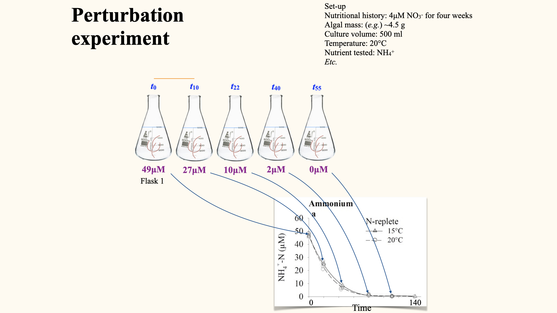
Perturbation experiments
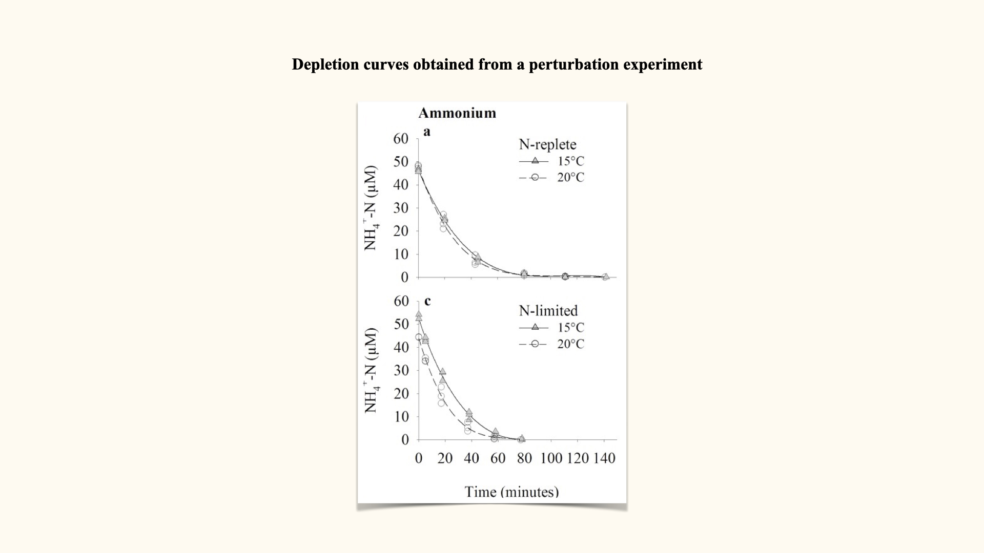
With the perturbation experiment (the approach used in your spreadsheet data you will encounter in the Lab), a single flask is set up with, for example, \(25\,\mu\mathrm{mol}\,\mathrm{L}^{-1}\) nitrate and a known mass of seaweed. At regular intervals (e.g., every five minutes), water samples are removed and nutrient content analysed. Rather than resetting the experiment for each time step, you use the same flask, tracking nutrient decline over time until it is depleted. The control flask should show no change, confirming the validity of the experiment.
This generates a depletion curve: plotting nutrient concentration over time, often for several replicate flasks at differing environmental conditions (e.g., high/low temperatures, pre-starved or already nutrient-replete seaweeds).
Caclculating depletion curves from perturbation experiments
The uptake rate, denoted \(V\), is the rate of nutrient uptake per gram per hour (or other unit of time). This is clearly shown in the depletion curves. Mathematically, it is the change in substrate concentration, \(\Delta Y\), over change in time, \(\Delta X\):
\[V = \frac{\Delta Y}{\Delta X}\]
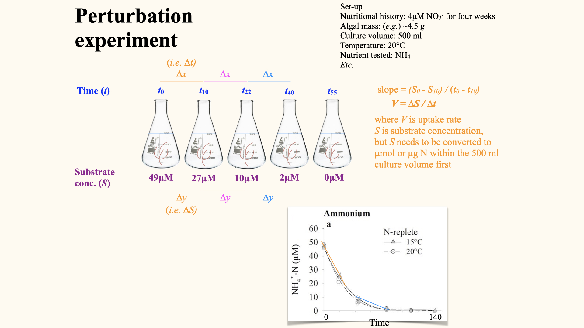
As you can see in the slide above, plotting a depletion curve is very straightforward. All you need to do is recognise that time is the independent variable; that is, it will be plotted on the x-axis. The nutrient concentrations remaining in the flasks after each consecutive time interval are plotted on the y-axis, which serves as the dependent variable. Once you have constructed the plot as I have just described, you will observe a curve very similar to the one I have shown for ammonium uptake.
For each time interval, you calculate this rate from the depletion curve. At the start — where the external nutrient concentration is highest — uptake rate is fastest, and the curve (shown above by the straight line fitted to the interval, whose slope is \(V\)) is steepest. As the nutrient is depleted, the curve flattens and \(V\) decreases.
Here is the sequence of steps, which are as logical and systematic as in the multiple flask experiments:
These rates (\(V\)) are then used for the next phase of analysis.
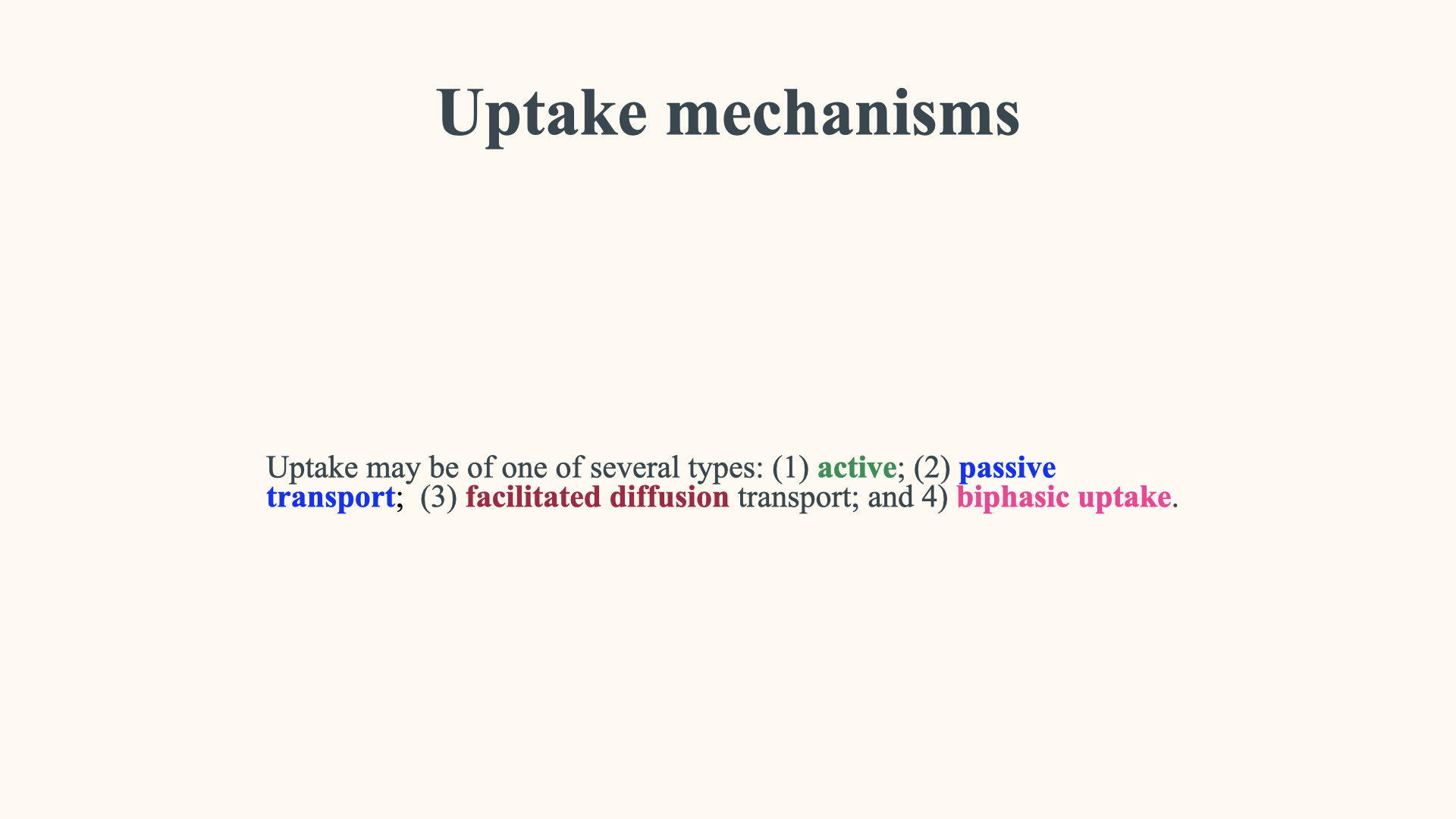
14 Different Uptake Mechanisms
Before we dive deeper into the calculation of uptake kinetics — in other words, kinetics meaning the study of the rate processes underlying some biological process — I think it is useful to distinguish between a couple of different ways in which seaweeds can take up nutrients.
There are four different kinds of nutrient uptake mechanisms. For the immediate sections following below, we will be talking about active uptake. In other words, this is a form of uptake where nutrient acquisition is driven by the expenditure of energy. This is typically the kind of uptake process that we study when we conduct multiple flask or perturbation experiments.
Another type of uptake — the second type — that we will cover later on in the lecture, which can also be studied by constructing depletion curves, is the process of passive transport or passive uptake. This is where nutrient uptake is entirely driven by processes involving the diffusion, the diffusive flux, of nutrients into the cells.
Much later on, we will talk, but not in too much detail, about facilitated diffusion transport and biphasic uptake.
For the next few sections in our lecture that continue below, the perturbation and multiple flask methods that we are applying will be showcasing how we would go about studying active transport. In other words, we will focus on cases where energy is expended to take up nutrients, and where the flux of these nutrients can proceed against the concentration gradient.
15 Uptake Kinetics: Michaelis-Menten Model
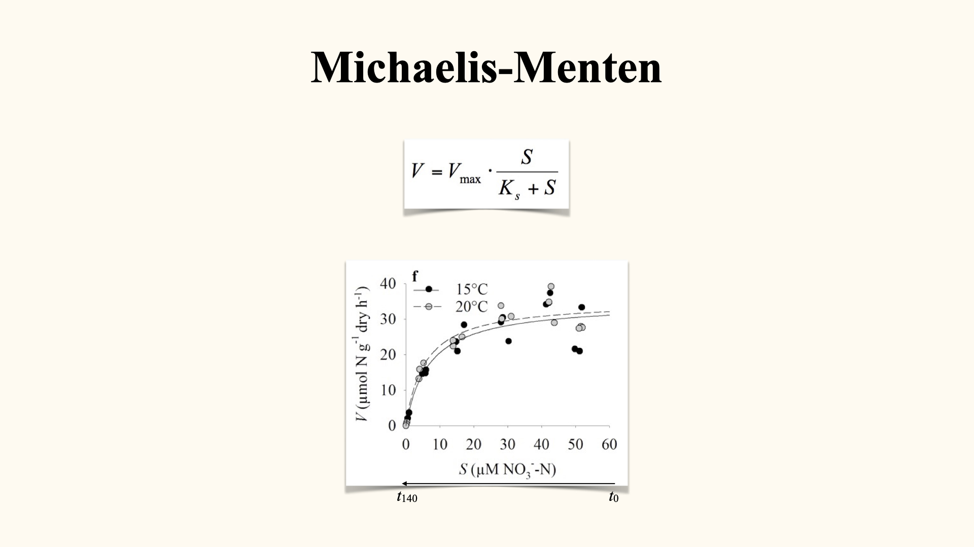
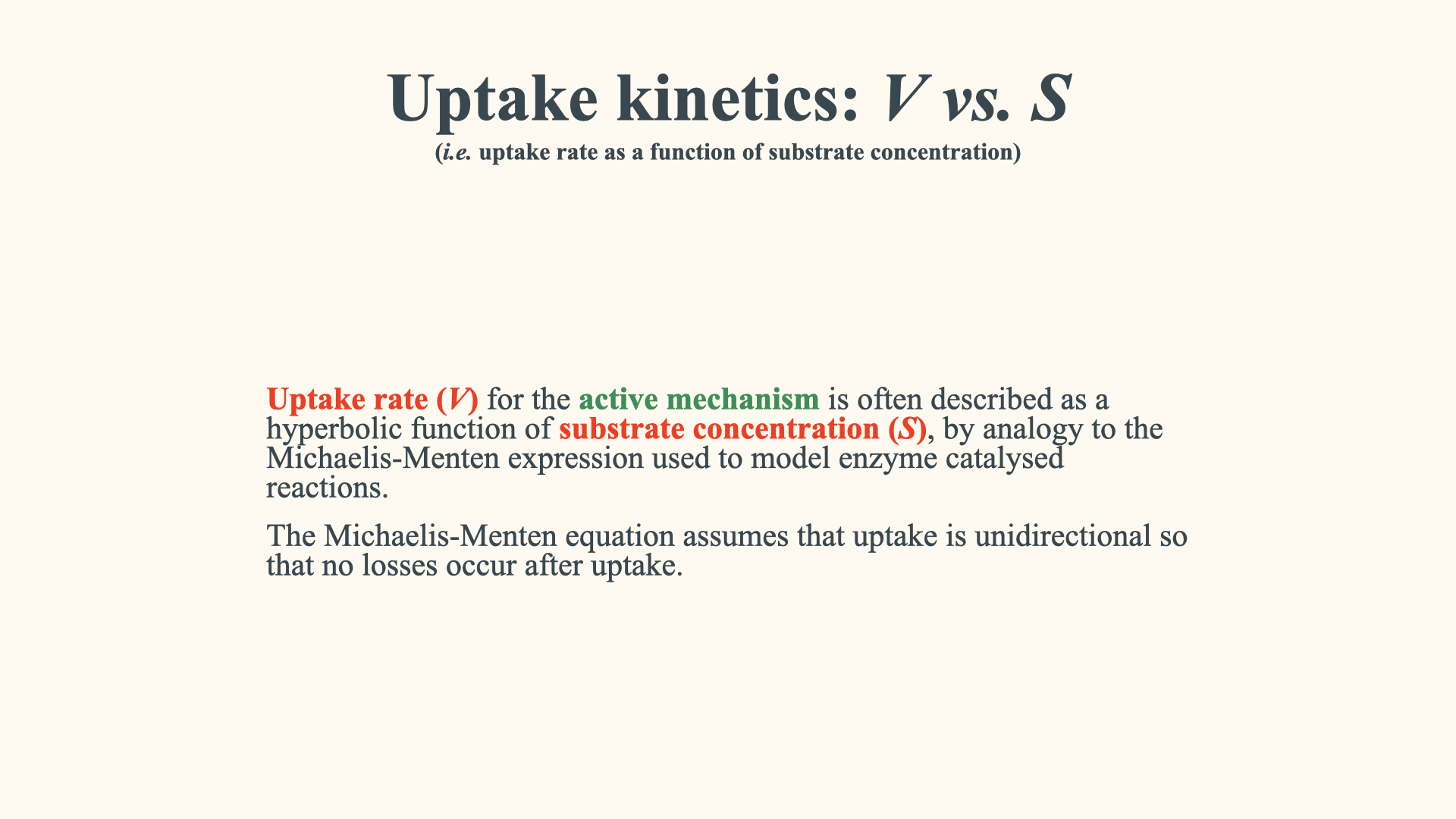
We then relate uptake rate (\(V\)) to the substrate concentration (\(S\)) we typically do so by generating a \(V\) vs. \(S\) plot. This relationship follows the Michaelis-Menten equation, familiar from enzyme kinetics, resulting in a characteristic hyperbolic curve:
- At high substrate concentrations (initially in the experiment), uptake rate is maximal and governed by the enzymatic processing capacity — the internal kinetic limit.
- As substrate is depleted, the rate drops off, and diffusion through the boundary layer becomes limiting — the external physical limit.
When plotting \(V\) against \(S\), we see:
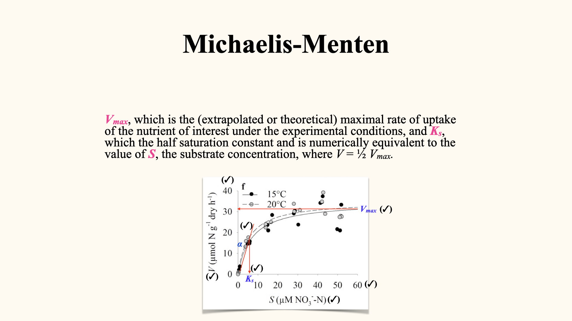
- A plateau at high external concentrations, where processes are enzyme-limited, called \(V_{\text{max}}\). It is important that, if seen as a time-related process, \(V_{\text{max}}\) occurs at the start of our experiment (in perturbation experiments), or as seen from the point of view of a multiple flask experiment, at the highest nutrient concentrations. In both instances, this is the slope of the line segments fitted to the start of our depletion curves.
- A curved downturn at lower concentrations, where diffusion and transport limitation take over, which is the process captured by the tail ends of the depletion curves (end of the process).
\[V = \frac{V_\text{max} \cdot S}{K_s + S}\]
Here, \(V_\text{max}\) is the maximum uptake rate (set by enzyme capacity), \(K_s\) is the half-saturation constant (substrate concentration at which \(V\) is half \(V_\text{max}\)), and \(S\) is substrate concentration.
When a graph of uptake rate (\(V\)) versus substrate concentration (\(S\)) displays a hyperbolic tangent curve — a steep rise at low concentrations and a plateau at high concentrations — this signifies active or facilitated uptake. The maximum rate of uptake (\(V_{max}\)) is primarily set by factors intrinsic to the algae, such as the enzymatic processes involved.
Consequently, environmental factors that influence enzyme activity — like light intensity or temperature — will impact how high \(V_{max}\) can be. Thus, active uptake is largely determined and influenced by environmental conditions that promote growth, photosynthesis, and metabolic activity — for example, high temperatures and abundant light.
15.1 Reading the Michaelis-Menten graph
At high \(S\), uptake is only limited by enzyme processing speed — even if you double or triple nutrients, \(V\) remains at \(V_\text{max}\). Once the environmental nutrients start to diminish, the rate \(V\) declines, indicating the transition to diffusion-limited uptake.
- \(V_\text{max}\)—maximal enzyme processing rate.
- \(K_s\)—substrate concentration where \(V\) is half \(V_\text{max}\), indicating the plant’s ability to extract nutrients at low concentrations.
- \(\alpha\) (alpha)—slope of the initial portion of the curve, reflecting affinity for nutrients in low-nutrient environments.
A low \(K_s\) (or steep \(\alpha\)) indicates high affinity, making certain algae better adapted to low-nutrient conditions. A high \(K_s\) suggests poor adaptation to nutrient poverty.
15.2 Applications and importance
Understanding these parameters helps explain why some seaweeds become opportunistic, blooming in nutrient-rich environments while others persist under nutrient limitation. The values of \(V_\text{max}\), \(K_s\), and \(\alpha\) are affected by species’ physiology, surface area to volume ratio, light, temperature, pre-conditioning, and other ecophysiological parameters.
You should now be able to connect plant ecophysiology and uptake models to the practical experiments and analysis required for your coursework. Remember to relate all elements back to both phases (diffusion and enzymatic reaction), and know which environmental or physiological factors are likely to limit uptake under different scenarios.
Right, so today we will continue to talk about nutrient uptake. Last week, we spoke about nutrient uptake experiments, and I showed you how to derive information from the depletion curve — the relationship that shows uptake rate versus substrate concentration. When we plotted that relationship, the graph appeared as a hyperbolic tangent curve. At low concentrations, the uptake rate increases rapidly, and then at high nutrient concentrations, it reaches a plateau. This type of relationship is known as the Michaelis–Menten uptake relationship, and it serves as an example of one of three different uptake mechanisms called active uptake.
On Thursday, we will discuss passive transport and facilitated diffusion, which are two additional uptake mechanisms. Generally speaking, algae and most other plants can display one of these three mechanisms — active transport, passive transport, and facilitated diffusion. Today, our focus will remain on active uptake.
Last week, after we explored the uptake curve — the \(V\) versus \(S\) relationship — of active uptake as determined for nitrate, I explained the various parameters: \(V_{max}\), \(K_s\), and \(\alpha\). On this slide, you will find text discussing the ecological significance of these parameters. We have covered this before, so I will not repeat it in detail. Instead, let us delve a bit further into what active uptake involves.
16 Active Uptake
Active uptake allows most plants to maintain nutrient concentrations inside their cells that are much greater than those found in the external environment. This process enables nutrients to be transported from an area where there is a lower concentration to an area inside the plant where there is a higher concentration — essentially moving against the concentration gradient. More formally, this occurs against the electrochemical potential gradient.
To quantify, external nutrient concentrations are usually in the micromolar range, while internal concentrations inside the cell are generally in the millimolar range — that is, from \(\mu\mathrm{mol}\,\mathrm{L}^{-1}\) externally to \(\,\mathrm{mmol}\,\mathrm{L}^{-1}\) internally. This large difference suggests that passive diffusion alone is insufficient, as diffusion would only allow movement from high to low concentration.
Passive diffusion is – at most – responsible for the movement of nutrients from the environment across the boundary layer. This specific process is determined by passive diffusion. However, the major uptake of nutrients into the cell is described by active uptake. For this to occur — from a region of low concentration to one of high concentration — cells must expend energy, namely metabolic energy.
The energy expended is generally light-dependent, with ATP being the most likely source. This is achieved by a system that involves proton-pumping ATPases, setting up a gradient between the external and internal environment in terms of pH. The proton gradient, or the pH gradient, establishes the electrochemical potential gradient, which then drives secondary ion transport. The secondary ion in question is the nutrient — such as nitrate, in our previous example.
This coupling between the pH gradient and the nutrient gradient facilitates the active uptake of nutrients. Coupled transport may arise from differing movements of ions at different sites, either in opposite or the same direction. When hydrogen ions are pumped out of the cell and nutrients are pumped in, this form of counter-transport is known as anti-port, or anti-porter transport. Conversely, some nutrients move in the same direction as the protons — this is called symport or co-transport.
In algae, the proton pump is linked to the co-transport of substances like sugars and thiourea, and there are also mechanisms involving the pumping of sodium ions, which can be responsible for the co-transport of other nutrients from the environment into the cell.
16.1 Key points of active uptake
You must remember that cellular energy, primarily derived from ATP, is required to drive active uptake. ATP drives the proton pump, which establishes the primary gradient, and then nutrients are brought into the cell by coupling to this gradient.
This is the mechanism by which an energetic, active process brings nutrients into the cell — by coupling with a proton pump generated by ATP and ATPases. While this is a complex physiological process, knowing this overview will suffice; we will not explore all the fine physiological details.
16.2 Characteristics that define active uptake
Beyond its energy requirement, active uptake is defined by several additional characteristics:
Selectivity for Particular Ions: Only specific ions are taken up via active transport, not all. For example, nitrate, phosphorus, and sulphates can be taken up in this way. One of the components of dissolved inorganic nitrogen (DIN), ammonium, is typically not taken up via active transport and is excluded here.
Saturation of the Carrier System: There is a stage in the uptake process where the carrier system becomes saturated. At high nutrient concentrations, there is a portion of the curve where \(V_{max}\) is reached — meaning uptake rate will not increase, despite increasing external nutrient concentration. This is because the enzymatic systems responsible for transport become saturated and cannot operate any faster.
Movement Against the Concentration Gradient: As previously discussed, active uptake involves the movement of ions against their concentration gradient.
When uptake rate (\(V\)) is plotted against substrate concentration (\(S\)) and the curve shows a steep initial rise followed by a plateau — i.e., a hyperbolic tangent shape — we can infer the process is mediated by either active or facilitated uptake. The maximum uptake rate, \(V_{max}\), is controlled by intrinsic factors within the algae, specifically those that govern enzyme function. Thus, environmental factors that influence enzyme activity, such as light intensity and temperature, will affect \(V_{max}\).
Put simply, environments promoting rapid growth — higher temperature, more light — will increase enzyme activities, resulting in a higher \(V_{max}\).
These features — selectivity, saturation, and movement against the gradient — define active uptake. Note that some of these factors also apply to facilitated uptake, which we shall discuss later.
16.3 Surface area to volume ratio and uptake parameters
Suppose we gather several seaweeds, spanning all six or seven different functional form categories outlined by Littler and Littler, and conduct uptake experiments. We would discover that \(V_{max}\) and \(K_s\) vary as a function of the surface area to volume ratio.
Plants with flat, membranous, or highly filamentous forms tend to grow rapidly and thus have a much higher \(V_{max}\)—thanks to their high surface area to volume ratio, which allows every cell direct exposure to the nutrient-rich environment. They are also typically able to acquire nutrients effectively even in environments where nutrient levels are low, implying they often have a low \(K_s\) (and thus a high affinity for nutrients).
On the other end of the spectrum, algae with a low surface area to volume ratio — where the bulk of the cells are internal — grow more slowly, with reduced access to light and slower diffusion rates. Consequently, they possess a low \(V_{max}\) and often a higher \(K_s\), making them less able to acquire nutrients when these are scarce.
If these low \(V_{max}\) species are placed in a nutrient-rich (eutrophic) environment, it makes little difference, because their limitation is set by internal cellular processes, not external nutrient supply. In contrast, fast-growing, high-surface-area species with high \(V_{max}\) and low \(K_s\) will respond rapidly to eutrophic conditions. This helps explain why some algae become nuisance or problematic under excessive nutrient conditions — their physiological traits make them well-suited to exploit high nutrient environments.
Understanding the ecological significance of high or low \(V_{max}\) and \(K_s\) is crucial; it explains the circumstances under which species will thrive and proliferate based on the environmental nutrient regime.
16.4 The three phases of active uptake
Active uptake can be described as having three phases:
- The Surge Phase
- The Internally Controlled Phase
- The Externally Controlled Phase
Let us discuss each in detail.
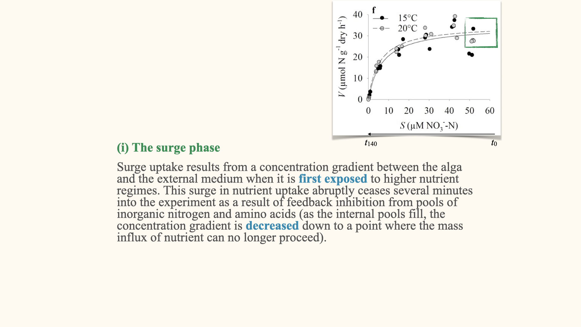
The surge phase
The surge phase is observed at the very beginning of nutrient uptake, at \(t = 0\). Imagine taking a seaweed that had not previously been exposed to nutrients and placing it into fresh seawater or a beaker with abundant nutrients. At the start, the environment is nutrient-rich, but the internal pools within the seaweed cells are nutrient-poor.
Immediately after exposure, there is a rapid influx of nutrients — nutrients rush into the cellular pools (like vacuoles) which had been depleted. Once the concentrations equalise, the surge phase ends. This rapid initial movement is the surge phase, driven by a steep concentration gradient.
The surge phase only occurs at the beginning of exposure to high nutrient concentrations. Once the internal pools are filled, the diffusive flux equalises, and the rapid uptake stops.
Note: Be mindful that, on the typical uptake curve, time runs in the opposite direction to substrate concentration; do not confuse the two.
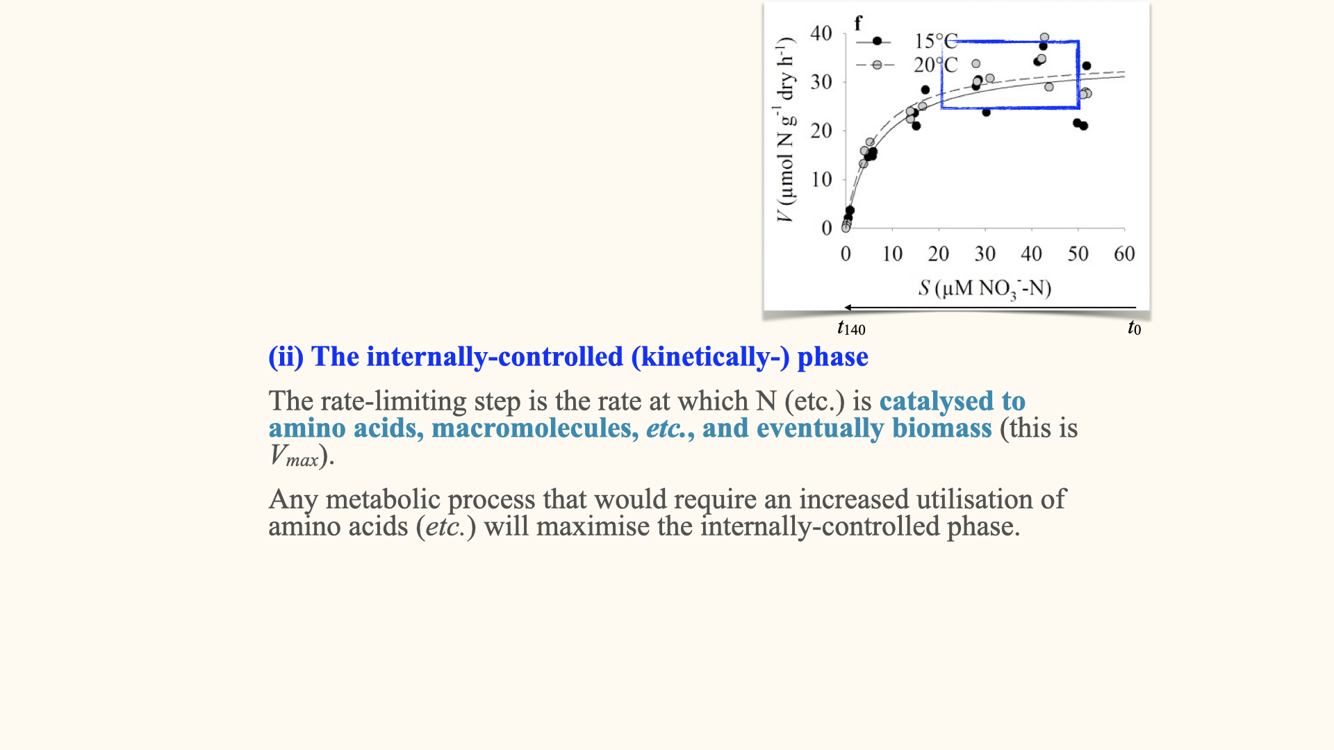
The internally controlled phase
After the surge phase, once the internal pools are filled, the rate of nutrient conversion — transforming inorganic nutrients already inside the cell into organic compounds (such as amino acids or other macromolecules)—becomes the limiting step. This is the internally controlled phase.
Here, the rate of nutrient uptake is governed by enzyme activity, and this phase sets the plateau seen in the uptake curve (\(V_{max}\)). The maximum rate is determined by how quickly the enzymes can process nutrients.
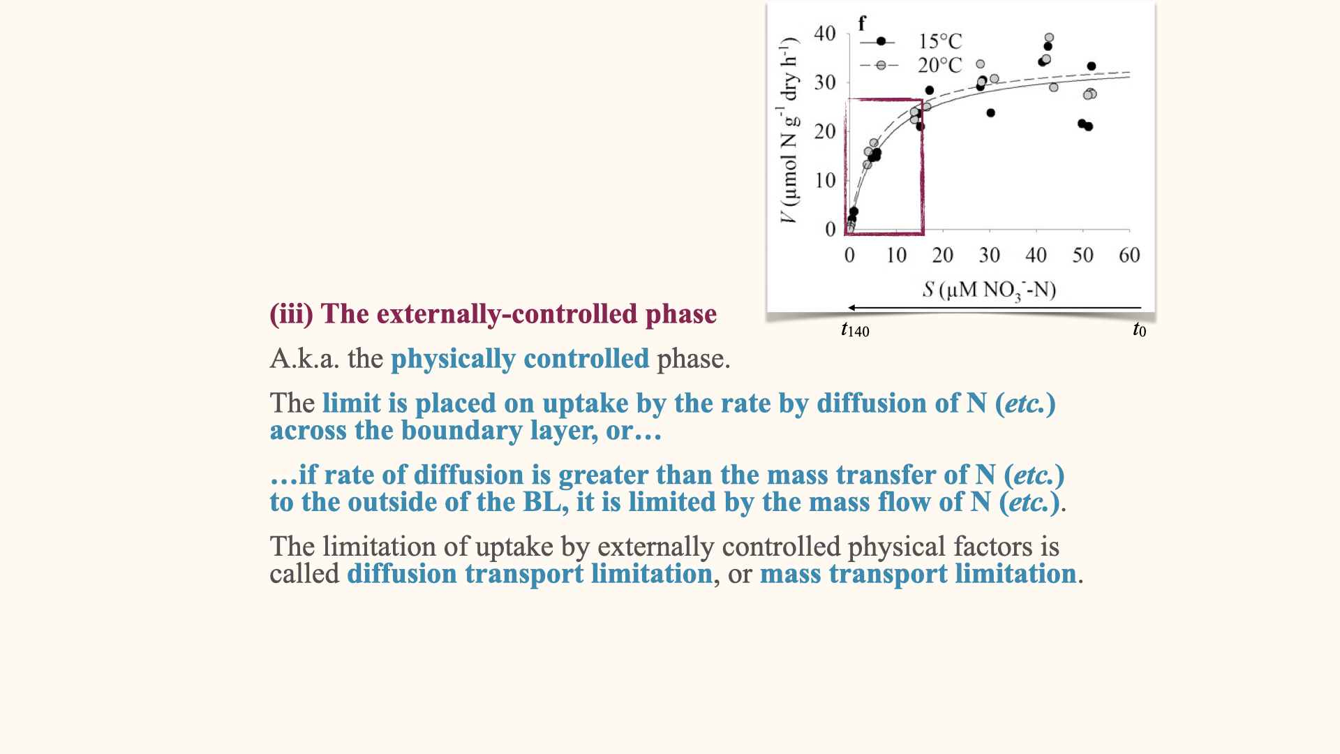
The externally controlled phase
If the plant remains in the closed environment and continues to take up nutrients, eventually the external nutrient concentration will drop. At some point, the uptake rate is determined by the diffusion of nutrients from the environment to the cell — this is the externally controlled phase.
At very low ambient nutrient concentrations, the uptake rate also becomes low, because diffusion is limited. As nutrient concentrations increase, the concentration gradient increases, and so does the diffusive flux. In this region, the rate of nutrient uptake is determined by the difference in concentration across the boundary layer surrounding the organism.
Two main factors influence the movement of nutrients across the boundary layer:
- The concentration gradient between the external environment and the cell.
- The thickness of the boundary layer, which is influenced by water movement; high water movement results in a thin boundary layer and hence faster diffusion, while low water movement causes a thicker boundary layer which slows diffusion.
All these external physical factors combine to influence the maximum rate of diffusion across the boundary layer.
16.5 Influence of morphology and environmental factors
Certain seaweeds with high surface area:volume ratios — those with flat, membranous, or highly branched forms — are optimised for rapid nutrient uptake. When placed in nutrient-rich medium, these forms respond almost instantly, with rapid increases in biomass, sometimes doubling mass within a day or two, given high \(V_{max}\) and sufficient nutrients.
On the other hand, seaweeds with significantly lower surface area:volume ratios respond more slowly. They may exhibit ‘luxury consumption,’ taking up nutrient amounts exceeding immediate growth requirements and storing these for future use when growth conditions permit.
Consequently, the physiological and morphological traits associated with fast uptake — high surface area:volume ratio, high \(V_{max}\), and low \(K_s\)—are precisely those that predispose certain species to become nuisance algae under eutrophic conditions.
16.6 Factors affecting nitrogen (and other nutrient) uptake
16.7 To summarise, several factors determine nutrient uptake rates:
- Physical environment: The concentration of nutrients in the water and the thickness of the boundary layer, affected by water motion.
- Form of nutrient: For example, ammonium is absorbed much more rapidly than nitrate. Nitrate must be taken up by active transport, whilst ammonium can diffuse passively into the cell.
- Nutritional state of the plant: Nutrient-starved plants will take up nutrients rapidly when re-exposed, while replete plants will not show a significant response.
- Growth environment: Higher light intensities and temperatures increase metabolic rates, raising \(V_{max}\) and thus enhancing nutrient uptake.
- Morphology: As discussed, a higher surface area to volume ratio increases both diffusion and uptake capacities.
- Uptake mechanism: Combinations of uptake mechanisms (active, passive, facilitated) determine overall absorption rates.
All of these factors interact to control the rate at which nitrogen, phosphorus, or any other macronutrient can be absorbed from the environment.
17 Passive Uptake
Good morning, everyone. This is our last lecture, so I would just like to wrap up more slides. It is not going to be a very long lecture. What we need to talk about today are the two remaining kinds of uptake mechanisms. We spoke at length about active uptake, which is characterised by the Michaelis-Menten equation, but there are also other kinds of uptake mechanisms, primarily passive uptake and facilitated uptake, and today we are going to quickly talk about both of those.
The reason why we have a different kind of uptake mechanism is because there are various different kinds of nitrogen available in the environment. For some of the more complex molecules like nitrate, active uptake is necessary, but there are more simple molecules also available that make up the total DIN (Dissolved Inorganic Nitrogen) pool, and in this instance we talk about the molecule ammonium or ammonia.
The passive uptake mechanism, when we talk about nitrogen uptake, is going to be mostly applicable to the uptake of ammonium from seawater into the seaweed itself. If you want to know a little bit more about nutrient uptake in seaweeds, and it is definitely recommended that you do this, you can read that paper that I wrote about 23 years ago in 2002, that talks about nutrient uptake, and it looks at nutrient uptake of ammonium and nitrate, and the various different rates of external water movement at different temperatures by one particular kind of seaweed. So have a look; it is going to give you nice additional extra information that is necessary, and that might make the difference in your exams, to be able to give me a mark, an answer worth 100% versus an answer worth 80%. So every little bit of additional work that you are going to do, by reading additional papers and so on, is going to count in your favour.
The uptake of ammonium is established in the same way that we do for nitrate uptake. In other words, we apply either multiple flask or perturbation experiments, we establish a depletion curve, and from the depletion curve we derive \(V\) versus \(S\), in other words the uptake kinetics graph.
When you plot the uptake kinetics graph for ammonium, you will notice that a straight line best describes the relationship between uptake rate and substrate concentration. Here we see a nice straight line going through all of the points. But in the instance at the bottom, when we look at the uptake of nitrate — also done via initially doing a depletion curve — and when we translate these data into those data, and we try and fit a line, we see that no longer can a linear relationship describe the relationship between \(V\) versus \(S\); it is mostly done via a Michaelis-Menten curve. But in passive uptake, when we try to relate \(V\) to \(S\), we are always going to find a linear relationship. That is the primary difference in the uptake kinetics between active uptake and passive uptake. Passive uptake, in the case of ammonium, is always going to give us, when we relate \(V\) to \(S\), a linear relationship.
This implies that in passive uptake, no expenditure of metabolic energy is necessary, because all of the uptake process can entirely be described by diffusion, and these usually involve the movement of uncharged molecules. Nitrate is a charged molecule because it has a negative charge; it is got some extra electrons. Ammonia, on the other hand, is a non-charged and uncharged molecule (as is CO₂, as is oxygen). So uncharged molecules usually diffuse from the external environment into the plant, down the concentration gradient, in other words, from where there is plenty of it in the external culture medium, to where there is less of it inside the plant. So it goes down the concentration gradient. In active uptake, it always goes against the concentration gradient, hence the necessity to use energy to drive that process.
Here, the entire thing relies mostly on diffusion, so therefore also processes external to the cell, external to the thallus, such as the rate of water movement that is going to have an influence on the thickness of that boundary layer, is going to be very important in affecting the rate at which the uptake can take place.
When we have a linear relationship – here we see the linear relationship – at no point along our increasing range of external concentrations (the substrate concentration) is there any evidence that the rate of uptake is going to slow down. With active uptake, the rate of uptake reaches a maximum, reaches a peak, which is \(V_\mathrm{max}\), but there is no \(V_\mathrm{max}\) here because it is a straight line. So if you are going to increase this concentration here from \(40\) to \(80\) to \(120\), the line is just going to continue to go up and up and up, which means that the rate of uptake is proportional to the amount of nitrogen present in the external environment only. That is going to set up higher concentrations, it is going to set up a steeper concentration gradient, and when we have a steeper concentration gradient, the rate of diffusion is going to increase.
That is what is meant here: the nature of the linear relationship means that we cannot, like in the case of the Michaelis-Menten relationship, calculate something called \(K_s\) or the parameter called \(V_\mathrm{max}\), because enzymes at no point, internal to the plant, have an influence on the maximum rate of uptake of these things. The \(K_s\) relationship, that point where the concentration that is associated with the rate of uptake, which is half of \(V_\mathrm{max}\), also cannot be calculated, because in order to calculate \(K_s\), we do need a \(V_\mathrm{max}\).
However, we can calculate a thing called \(\alpha\), and \(\alpha\), in the case of a linear relationship, is simply the slope of that line. The slope of the line is directly related to \(\alpha\) – it is \(\alpha\), in fact – so by simply calculating the slope of a linear regression, we can know what \(\alpha\) is, and \(\alpha\) has the same meaning as in the case of active uptake: it tells us something about the affinity of the plant for a particular nutrient. In other words, the steeper \(\alpha\) is, the more rapidly uptake rate is going to respond to a change in nutrient concentration. But with a low \(\alpha\) (in other words, a very shallow slope), you need a far larger change in nutrient concentration for it to bring about the same rate of change in uptake rate.
So things with a very steep \(\alpha\), a very steep curve, will show a kind of seaweed that is very able to take up nutrients when the amount of nutrients in the external environment is low. Seaweeds generally with a low \(\alpha\) – sorry, a, yes, a less steep slope, in other words, a low \(\alpha\) – those are the kinds of seaweeds that if you put them in a low nutrient environment, they are not going to be able to take up nutrients very effectively. Usually, given a particular nutrient concentration, say a nutrient concentration that is very low, and you put a seaweed with a low \(\alpha\) right next to a seaweed with a high \(\alpha\) in the same low nutrient water, the seaweed with a high \(\alpha\) is going to be better able to take nutrients from that seawater, and is better able to sustain its nutritional needs in order for it to continue to grow when the environmental nutrient concentrations are low.
So that is a nice way that you can use the knowledge of the steepness of that slope – in other words, that mathematical relationship that relates the rate of uptake to the amount of nutrients present in the water – that knowledge tells us something about the ecological competitiveness of two different kinds of seaweeds with different alphas in the same nutrient medium. And this also tells us a little bit about which seaweeds are going to become more prone to becoming nuisance seaweeds under eutrophic conditions. So the ones with a high \(\alpha\) are going to be the ones that are also going to be able to respond very rapidly to any enhanced amount of nutrients in the environment, and they are going to have a tendency to become a nuisance species when eutrophication happens.
17.1 Uptake kinetics and the affinity coefficient
So, when we have a linear relationship — for example, in passive uptake — at no point along our increasing range of external substrate concentrations is there any evidence that the rate of uptake slows down. In active uptake, the rate of uptake reaches a maximum, which is \(V_{\text{max}}\), but in passive uptake, there is no \(V_{\text{max}}\), because it is a straight line. If you increase the substrate concentration from \(40\) to \(80\) to \(120\), the line will just continue to go up, which means that the rate of uptake is proportional to the amount of nitrogen present in the external environment.
A higher external concentration sets up a steeper concentration gradient, and when we have a steeper concentration gradient, the rate of diffusion increases. This is why, in a linear relationship, we cannot, as we do in the case of Michaelis-Menten kinetics, calculate the parameters \(K_s\) or \(V_{\text{max}}\), because enzymes at no point, internal to the plant, influence the maximum rate of uptake in these cases. And the \(K_s\) relationship — that is, the substrate concentration at which uptake rate is half of \(V_{\text{max}}\)—also cannot be calculated, because in order to calculate \(K_s\), we need a \(V_{\text{max}}\).
However, we can calculate a parameter called \(\alpha\), and \(\alpha\), in the case of a linear relationship, is simply the slope of that line. The slope of the line is directly equal to \(\alpha\), so by calculating the slope from a linear regression, we can know what \(\alpha\) is. Alpha has the same meaning as in the case of active uptake: it tells us about the affinity of the plant for a particular nutrient.
So, the steeper the \(\alpha\), the more rapidly the uptake rate increases with a change in nutrient concentration. By contrast, with a low \(\alpha\), or a very shallow slope, you need a far greater change in nutrient concentration to produce the same change in uptake rate.
Seaweeds with a steep \(\alpha\)—that is, a steep curve — are able to take up nutrients efficiently, even when the amount of nutrients in the external environment is low. Seaweeds with a low \(\alpha\)—a shallow slope — will not take up nutrients effectively in low-nutrient environments. So, given a particular low nutrient concentration, if you put a seaweed with a low \(\alpha\) next to one with a high \(\alpha\) in the same water, the one with the high \(\alpha\) will better sustain its nutritional needs and enable continued growth in those conditions.
This is a useful way to use knowledge of the steepness of that slope — in other words, the mathematical relationship that relates uptake rate to nutrient concentration in the water. This knowledge tells us about the ecological competitiveness of two different seaweeds with different alphas, in the same nutrient medium. It also tells us something about seaweeds likely to become nuisance species under eutrophic conditions. Those with a high \(\alpha\) can respond rapidly to increased nutrient availability, and may become nuisance species when eutrophication occurs.
17.2 Passive uptake, thallus morphology, and the monod equation
In seaweeds that are predominantly governed by passive uptake, where the main process driving nutrient acquisition is diffusion, we find that their thallus morphology is typically defined by a highly elevated surface area to volume ratio. In such organisms, many — if not all — of the cells are in direct contact with the external environment. As a result, there is very little capacity for the formation of complex internal tissues capable of storing nitrogen in forms such as the various nitrogenous storage compounds, for instance, phycobilins, phycobiliproteins, or other proteins.
This morphological adaptation means that nitrogen taken up via rapid diffusion — owing to the high surface area to volume ratio — immediately supports growth. The process is such that nutrient uptake directly and instantaneously leads to biomass accumulation. In these situations, we characterise the relationship between the growth response and the preceding nutrient uptake rate as a very tight, direct, linear coupling.
This relationship does not imply that growth increases indefinitely as nutrient concentration rises. At some point, growth becomes limited by the internal machinery of the organism. Diffusion may still deliver nutrients rapidly, but biomass production cannot exceed the maximum rates at which the relevant enzymes and cellular processes operate.
So, beyond certain environmental nutrient concentrations, where growth and nutrient uptake are linear, further increases in nutrient concentration will see the growth rate begin to slow down. This is quite similar to what we observe in the Michaelis-Menten uptake response, where the uptake rate slows down at very high nutrient concentrations. This type of relationship, which couples the growth response to environmental nutrient availability, is described by the Monod equation. Functionally, it is quite similar to the Michaelis-Menten equation. The only significant difference is that, whereas the Michaelis-Menten equation shows \(V_{\mathrm{max}}\) or \(V\) as a function of substrate concentration, \(S\), the Monod equation describes growth rate as a function of \(S\).
These particular seaweeds, with their morphological and physiological adaptations, are especially prone to become problematic during eutrophication events. Because there is such an immediate translation of nutrient enrichment to growth, they can respond very quickly to increased ambient nutrient concentrations and thus proliferate rapidly.
By contrast, in the alternative scenario — where growth is not instantaneously stimulated following nutrient addition — we observe a phenomenon known as luxury consumption. In this mode, nutrients are taken up and stored internally within the seaweed as molecular forms that contribute little to immediate biomass increment. Instead, these stored forms serve principally as a reservoir of nitrogen.
Typically, seaweeds engaging primarily in active uptake fall into this category. The nutrients stored internally can subsequently be re-mobilised during periods when ambient nutrient concentrations decline to sufficiently low levels such that further influx by diffusion or active uptake is heavily constrained. In this way, the seaweed can continue to support growth by drawing upon its internally stored nitrogen reserves, even when external supply is insufficient.
18 Facilitated Uptake Mechanism
The third type of uptake, after active and passive, is facilitated uptake. Facilitated uptake resembles passive uptake in that it moves nutrients down a concentration gradient — the external concentration is greater than inside the cell.
However, unlike passive uptake, which relies entirely on diffusion, facilitated uptake uses a particular membrane protein that spans the cell membrane. This protein has an orientation across the membrane; its active site is external to the plant and specific for a particular molecule — say, for instance, sulphate. It binds to the sulfate outside, then flips around and releases it inside the cell.
In short, a protein collects something from outside, flips its conformation, and releases the molecule inside the cell — this is facilitated uptake. It is similar to passive uptake in being down the concentration gradient, but it is also similar to active uptake in showing a saturation response. That is, there is a maximum external concentration beyond which the transport protein cannot increase the rate of transport further — there is a \(V_{\text{max}}\). Facilitated uptake is also very specific to particular nutrients, and is susceptible to competitive and non-competitive inhibition. For example, another molecule may compete with the primary substrate (such as sulfate) for the active site, displacing sulphate and preventing its uptake.
That is essentially what facilitated uptake is about, and I will not go any further on that point.
19 Biphasic Uptake
We begin with the idea of biphasic uptake. The term refers to a two-phase response in the way algae absorb nutrients, depending on how much of the nutrient is available in the environment. What makes this process interesting is that it is not a fixed, rigid pattern — it is an adaptive strategy. By switching between modes of uptake, algae can remain flexible across very different nutrient environments. In nutrient-limited waters, they prioritise efficiency: they use high-affinity systems that allow them to extract and hold onto scarce nitrogen. But when nitrogen is plentiful, the strategy changes. High-affinity uptake, which is energetically costly, becomes unnecessary, and the cells may downregulate these systems to conserve energy, relying instead on lower-affinity mechanisms. In this sense, biphasic uptake reflects a balancing act between efficiency and economy, depending on the ecological context.
If we contrast this with other uptake patterns, the distinctiveness becomes clearer. Many organisms follow a hyperbolic uptake curve, where uptake rises with nutrient concentration but tends to level off — following Michaelis-Menten kinetics. A linear uptake pattern, by contrast, can occur under steady nutrient supply, where uptake increases proportionally with concentration, often constrained by diffusion or simpler transport processes. The biphasic form is more dynamic. It reflects an ecological adjustment: rather than following a single trajectory, algae switch gears when the nutrient environment changes. This allows them to optimise both metabolic costs and the efficiency of resource acquisition — an economy of effort matched to conditions.
Looking more closely, we can describe the two phases in detail. In the first phase — the high-affinity phase — the system dominates when nutrients are scarce. Uptake increases sharply even at very low concentrations, a response driven by specialised transport proteins with high binding affinity. This is an energetically demanding mode of absorption, but it is also the only way to secure survival when resources are scarce.
The second phase — the low-affinity or saturation phase—develops as concentrations increase. Uptake rates slow, often plateauing, because the cell no longer needs to operate at maximum efficiency. Here, uptake can become more passive, sometimes resembling diffusion, and the cell expends less energy. Additional transport proteins may be employed, but they typically have lower affinity and higher capacity, fitting environments where nutrients are abundant.
Together, these two modes exemplify a flexible ecological design. The biphasic uptake pattern underscores how algae are not passively subject to nutrient conditions but actively restructure their uptake machinery. By doing so, they maintain competitiveness across the shifting gradients of their environments.
20 Factors Modifying Uptake Rates
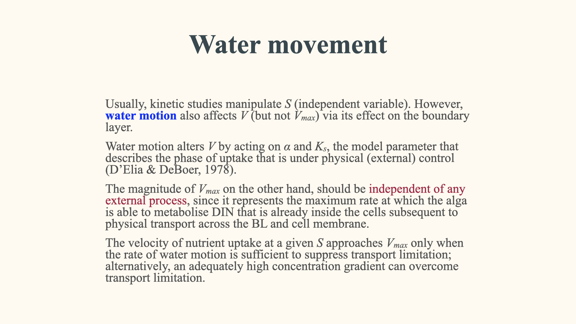
20.1 Water movement
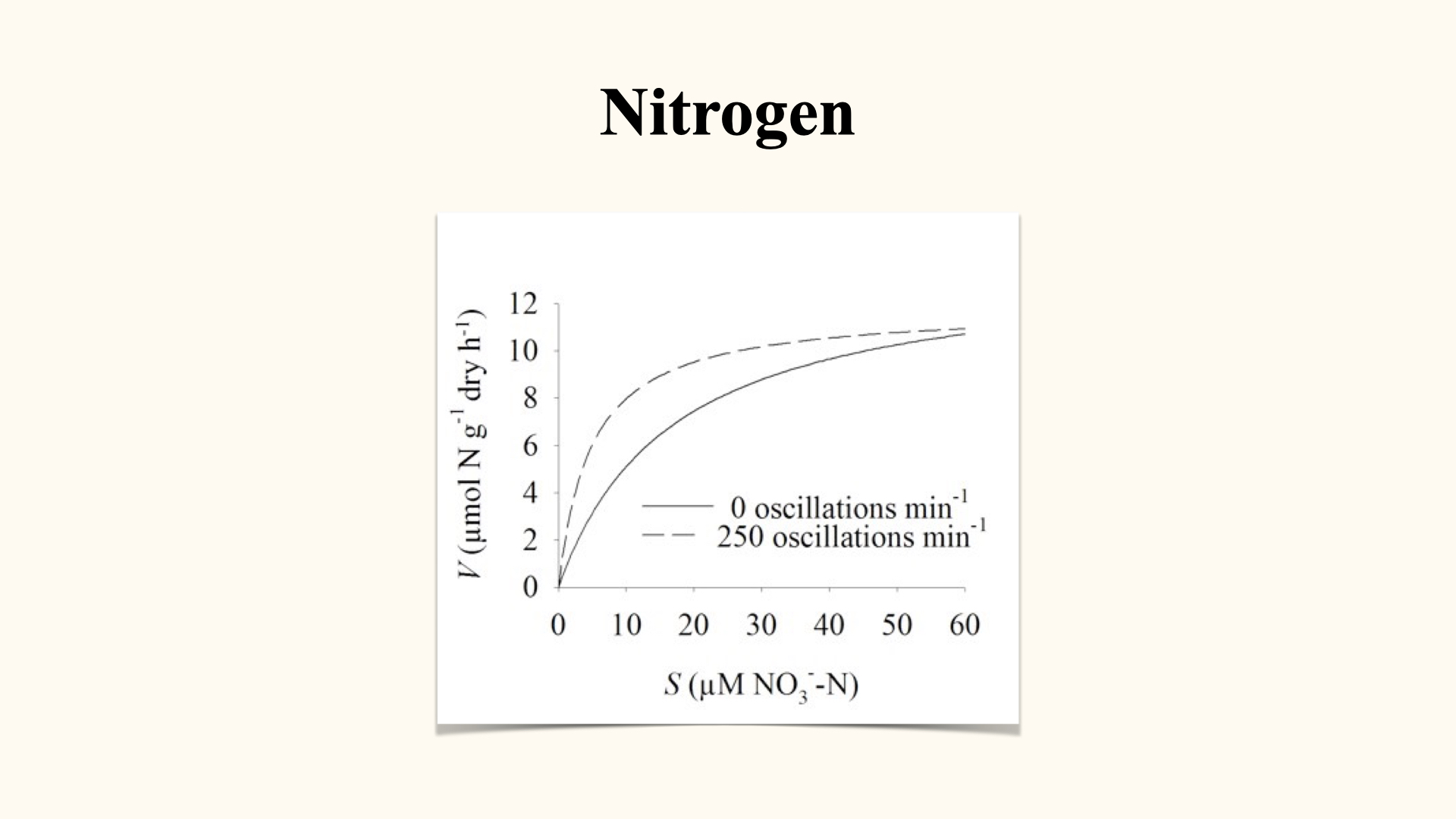
Water movement is a important environmental variable. Consider the ocean: it is highly variable in terms of waviness and the water movement occurring both at the surface and underwater, particularly around seaweeds. Depending on the rate of water movement, there will be a direct effect on the ability of seaweeds to take up nutrients.
Water movement primarily affects the rate parameters—\(V\), the rate of uptake, \(\alpha\), and \(K_s\)—but it does not influence \(V_\mathrm{max}\), the maximum rate at which nutrient uptake can occur. \(V_\mathrm{max}\) is always governed by processes operating within the plant itself. In contrast, water motion impacts processes occurring outside of the plant, altering uptake rates via two mechanisms.
The first mechanism is the reduction in the thickness of the boundary layer. A thick boundary layer typically acts as an impediment to nutrient acquisition. With high rates of water movement, the boundary layer becomes thinner, thereby reducing the friction, or resistance, across the interface of the cell wall and the external environment.
The second mechanism is related to the replenishment of localised nutrient depletion. As nutrients are drawn from the immediate vicinity of the seaweed and absorbed into the cells, this can result in a zone of reduced nutrient concentration adjacent to the seaweed. Water movement helps to replace these depleted nutrients — one of the only mechanisms by which this can occur — by enhancing the flow and bringing in new water with a higher concentration of nutrients to occupy the space previously lacking.
Let us consider the effect of water movement on nutrient uptake. To demonstrate this, examine the graph presented here, which contains two traces — one depicted as a dashed line and the other as a solid line.
The dashed line represents nutrient uptake in an experiment where glass containers are placed on a shaker table operating at \(250\) oscillations per minute, intended to emulate an environment with significant water movement. This setting mimics the rate at which water might move around seaweeds in more dynamic aquatic habitats. In contrast, the solid line reflects a condition set to zero oscillations per minute, meaning the water is completely static — absolutely still, with no movement at all around the seaweeds.
Now, if you observe the dashed line, corresponding to \(250\) oscillations per minute, you will note that both the rate parameters \(K_s\) and \(\alpha\) shift. Specifically, \(K_s\) decreases to a lower value, and \(\alpha\) increases to a higher value. Both of these changes indicate that the rate of diffusion — and therefore nutrient uptake — is significantly enhanced under conditions of elevated water movement.
Conversely, the zero oscillations per minute trace clearly demonstrates a pronounced boundary layer effect. Due to this strong boundary layer, the value of \(K_s\) is increased, and the initial slope of the uptake curve, \(\alpha\), is also rather low. Together, these parameters provide clear evidence of the diffusive resistance to nutrient uptake that operates under still water conditions.
20.2 Nutritional history
Typically, when we expose seaweeds – I have already mentioned this in some previous lectures – to a high concentration of nutrients and they continue to be present within that high concentration of nutrients, their rate of uptake is going to slow down because there is no need for them to take up nutrients since all the nutritional requirements have already been met.
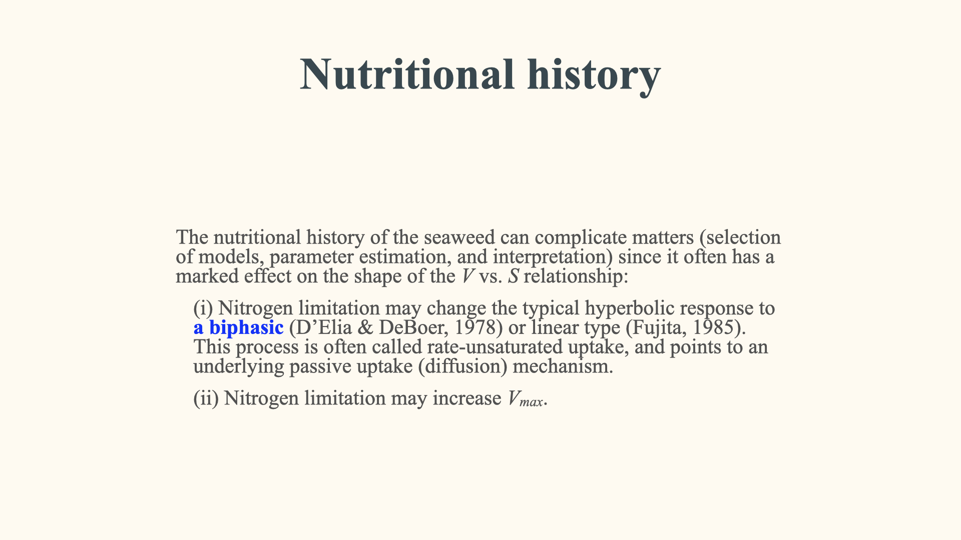
But if you take a seaweed from oligotrophic conditions and you remove it from that water and you put it into a new bucket of water with more nutrients in it, it is going to have a very rapid rate of uptake. That is going to increase, in the case of active uptake, it is going to increase the \(V_\mathrm{max}\). In the case of passive uptake, it is going to have an influence on the steepness of that line, in other words, \(\alpha\). So the more deprived something is of nutrients, the more it is going to respond in terms of rapidly taking up nutrients when it is placed into an environment where nutrients are quite available.
That is one of the ways in which seaweeds are going to respond to conditions or situations that are going to have a modification on the rate parameters we can estimate from either a linear curve or from a Michaelis-Menten kind of relationship.
In the case of active uptake, this can increase \(V_{\text{max}}\). In passive uptake, this influences the steepness of the line—\(\alpha\). The more deprived a seaweed is of nutrients, the greater the response in uptake when exposed to higher nutrient levels.
20.3 Light intensity and photoperiod
Another important factor is the light environment. What photosynthesis does is it takes inorganic carbon and puts it inside of the plant and makes it available, converts it into organic carbon. But in order for organic carbon to be also present as an organic molecule, it needs to be coupled with nitrogen. Remember, organic molecules are always molecules that have in the same molecule, generally, carbon, hydrogen, oxygen, nitrogen, phosphorus; all of those need to be present in order for it to be called an organic molecule. So in order for an organic molecule to be formed inside of the plant, the carbon that is taken up and whose rate of uptake is enhanced under high light conditions, once you put more organic carbon into the plant, it is going to need more nitrogen in order for it to produce organic molecules. So when something produces more carbon, the need for nitrogen uptake increases.
Therefore, typically, when you put a plant into a high light environment or a dim light environment, the ones that are in the high light environment are going to have a higher nutrient uptake rate compared to the ones in dim light. The reasons are explained there. This is true for both linear (passive) and active uptake – more light generally means more rapid photosynthesis.
In the case of active uptake, this is mostly going to affect the rate parameter \(V_\mathrm{max}\). Coming to linear uptake responses, for passive uptake, the more light there is, the more rapid the rate of photosynthesis is going to be (steeper slope).
Another reason is photoperiod. In other words, whether it is day or night, or how long the light period is compared to the amount of night-time that is available, because the enzyme nitrate reductase – that is the enzyme that is first going to take nitrate once it has been taken up and convert it into ammonium before the ammonium can be translated into amino acids – that activity of the nitrate reductase enzyme is very much coupled to photoperiod. So the more light there is, the more active nitrate reductase is going to be, and the faster the rate of nitrate uptake during light conditions. So with longer light availability, nitrate reductase is more active, and therefore the rate of nitrate uptake is greater.
20.4 Temperature
Another thing is, of course, temperature. I have mentioned this also before. That is because of this thing that is called \(Q_{10}\). This is something that Prof Maritz must have mentioned in one of his lectures when he talks about the rate of metabolism, and typically the rate of metabolism doubles for every \(10^\circ\mathrm{C}\) increase in temperature. As the rate of metabolism increases as a function of temperature, it means that more organic carbon can be formed, and as more organic carbon can be formed, it requires more nitrogen to be taken up. Because things grow faster – obviously up until the optimal or maximum temperature – when they grow faster as a result of being exposed to more heat, more nitrogen would also be necessary for it to support the formation of organic molecules.Temperature effects tend to be ion-specific and depend also on the species, so it is going to depend on whether it is taking up nitrate or ammonium, and this effect of temperature to enhance the rate of metabolism is going to very much depend upon the species in question.
20.5 Nutrient type
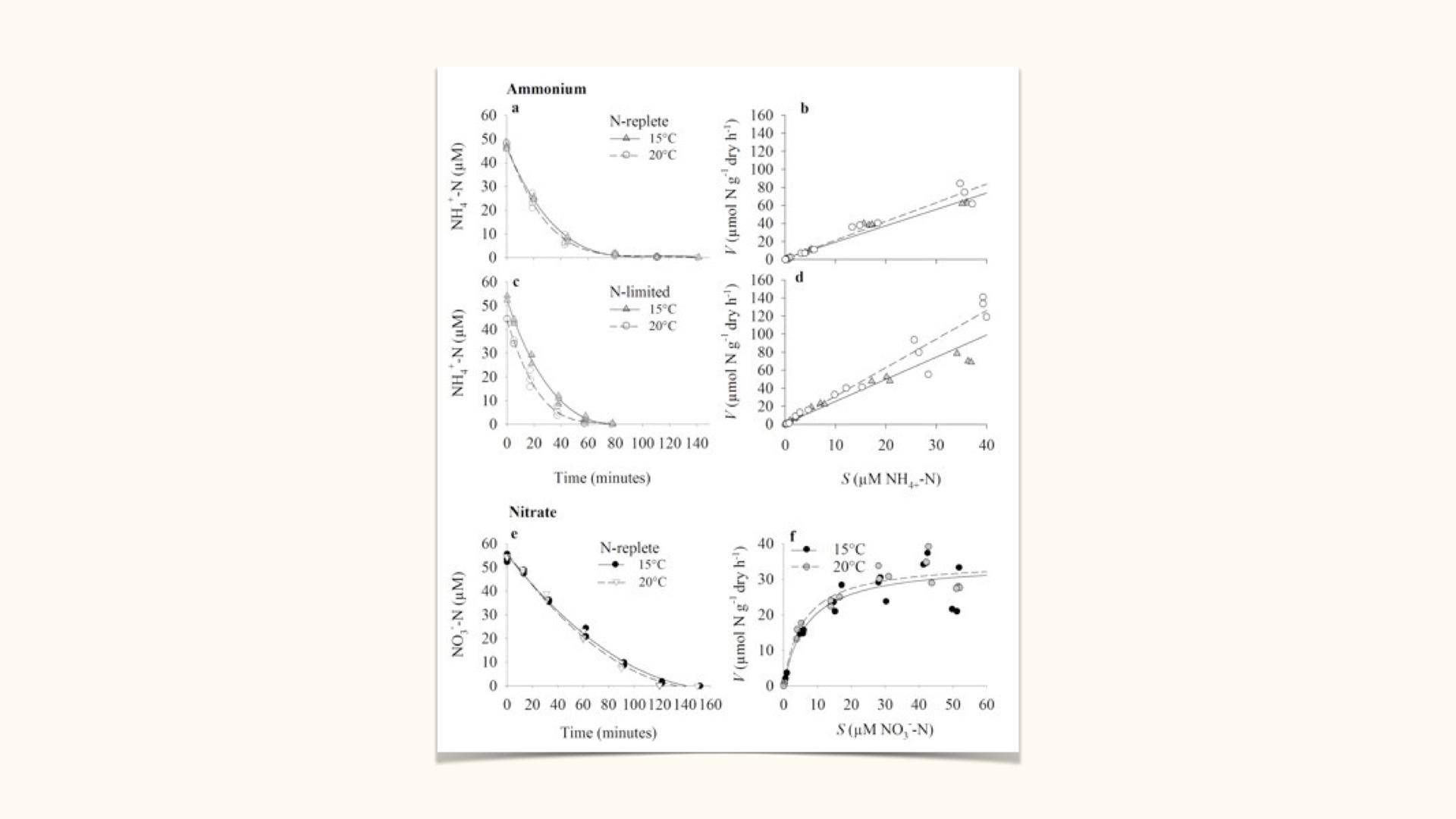
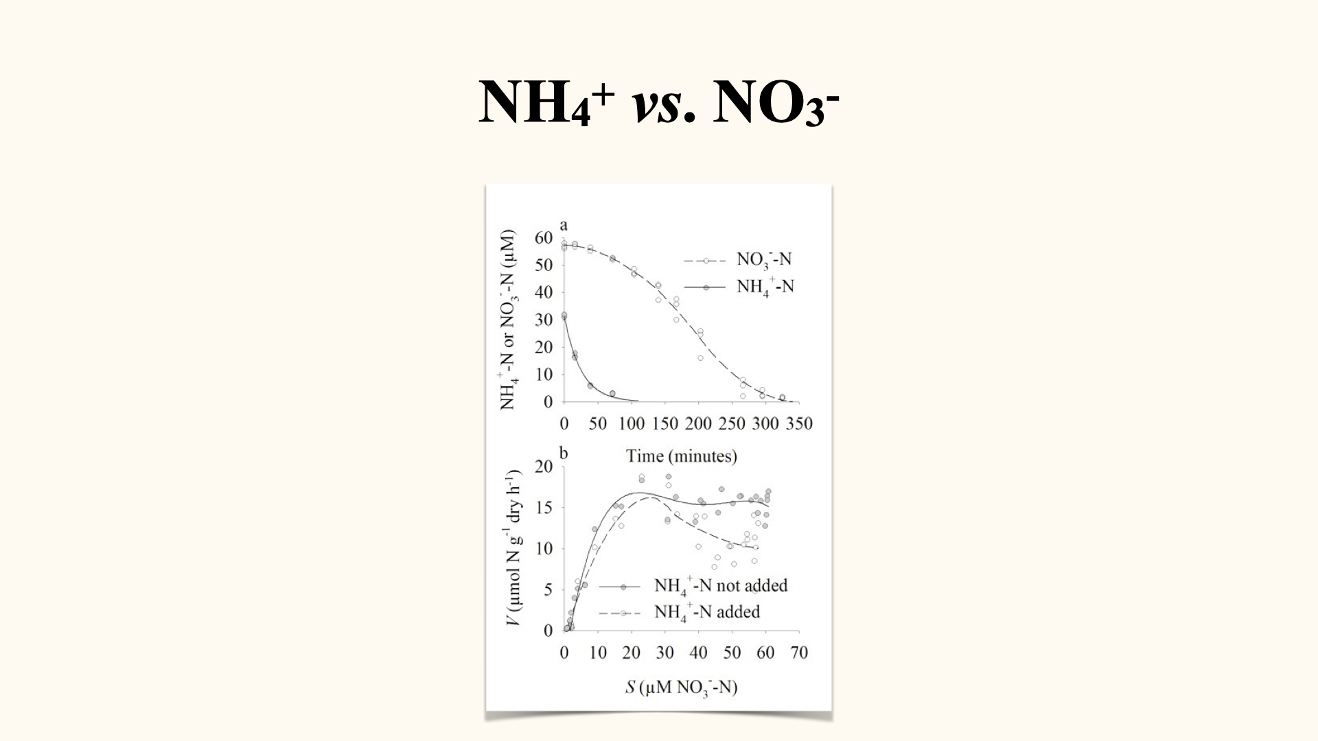
The type, and the concentration of nutrients also play a role. For instance, the type of nutrient — ammonium versus nitrate — dictates uptake mechanism: ammonium shows a linear, passive mechanism, while nitrate shows a Michaelis-Menten active mechanism.
Some nutrients interact in their uptake. If ammonium and nitrate are both present in culture medium, seaweeds will preferentially take up ammonium; nitrate uptake does not occur until all ammonium has been depleted.
20.6 Other factors
Other influences include surface area to volume ratio. You need to know, in detail, how the surface area to volume ratio modulates different physiological responses in seaweeds.
There are also various different intrinsic adaptive biological factors, such as the production of hairline hairs. Sometimes some seaweeds, under very oligotrophic conditions, would actually physiologically enhance or change their morphological appearance, and they do this by producing hairline hairs. Hairline hairs are just small little protrusions from the surface of a normally flat algal thallus. As it produces little hairline hairs, it increases the surface area to volume ratio and increases the affinity for nutrients. Therefore, the seaweed becomes more effective at taking up nutrients when the environmental nutrient concentrations are low.
There are also things such as the reproductive state. Some seaweeds, when they become reproductive, would require an enhanced uptake of nutrients in order to sustain gamete and spore production. Sometimes as a seaweed thallus ages into something that is older and grows slower, the rate of nutrient uptake would decrease with time. When it is very young and rapidly growing, the rate of nutrient uptake would have to be high. Sometimes there are seaweeds that change between morphological appearance — they have heteromorphic alternations of generations. One morphological appearance of a seaweed would have a different kind of nutrient uptake response compared to the other morphological appearance in the same species. There can also be, within the same species, different genetic influences that can affect the uptake kinetics of seaweeds.
21 Conclusion
If you need to know more about seaweed nutrient uptake, or nutrient uptake more generally (which can be generalised to plants), do look at the references provided. At the very least, I would like you to read the paper I wrote, as everything I have lectured on around this section is based on those experiments.
And that brings me to the end of this nutrient uptake lecture, and indeed to the end of BDC223 as far as the plant component is concerned.
Reuse
Citation
@online{smit2024,
  author = {Smit, A. J. and J. Smit, A.},
  title = {Lecture 8a: {Nutrient} {Uptake}},
  date = {2024-09-18},
  url = {https://tangledbank.netlify.app/BDC223/L08a-nutrient_uptake.html},
  langid = {en}
}