BCB744 BioStats 2025 Example 1

Author

Affiliation

Smit, A. J.

University of the Western Cape

Please download the data files required for this exercise from Google Drive (link provided by email). The files include:

• tmax.2016.nc – NetCDF file containing daily maximum temperature data for the year 2016.
• tmin.2016.nc – NetCDF file containing daily minimum temperature data for the year 2016.
• precip.2016.nc – NetCDF file containing daily precipitation data for the year 2016.
• All files in the subdirectory Studyarea – shapefiles of the study area.

Instructions

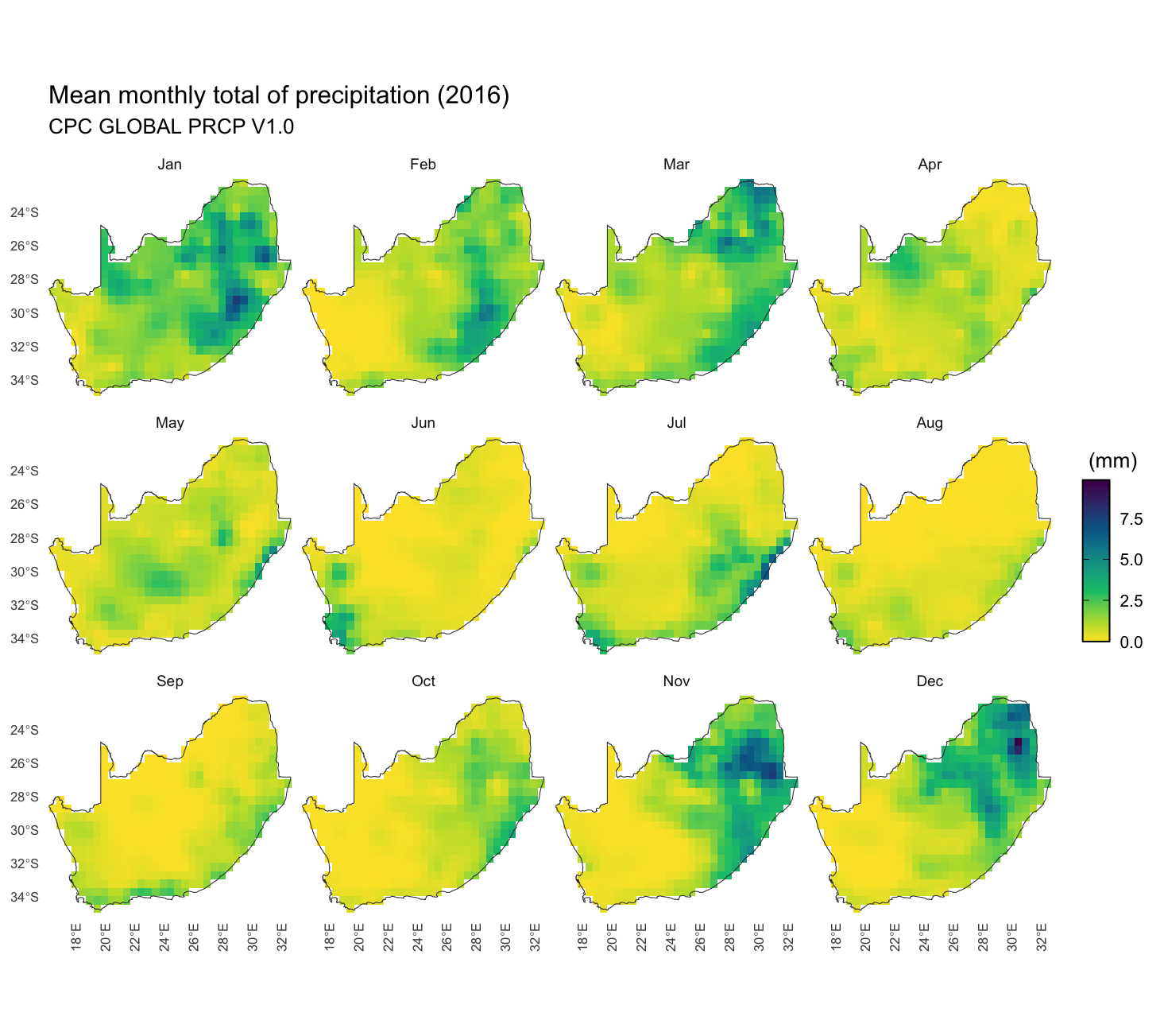
1. Load the precipitation data and calculate the mean monthly precipitation from the daily precipitation values, as well as the mean monthly value from the daily $\sqrt{precipitation}$.
2. Load the temperature data and calculate the mean monthly temperature from the daily $(t_{max}+t_{min})/2$, as well as the mean monthly value from the daily $\sqrt{(t_{max}+t_{min})/2}$.
3. Merge temperature and precipitation data into a single data frame.
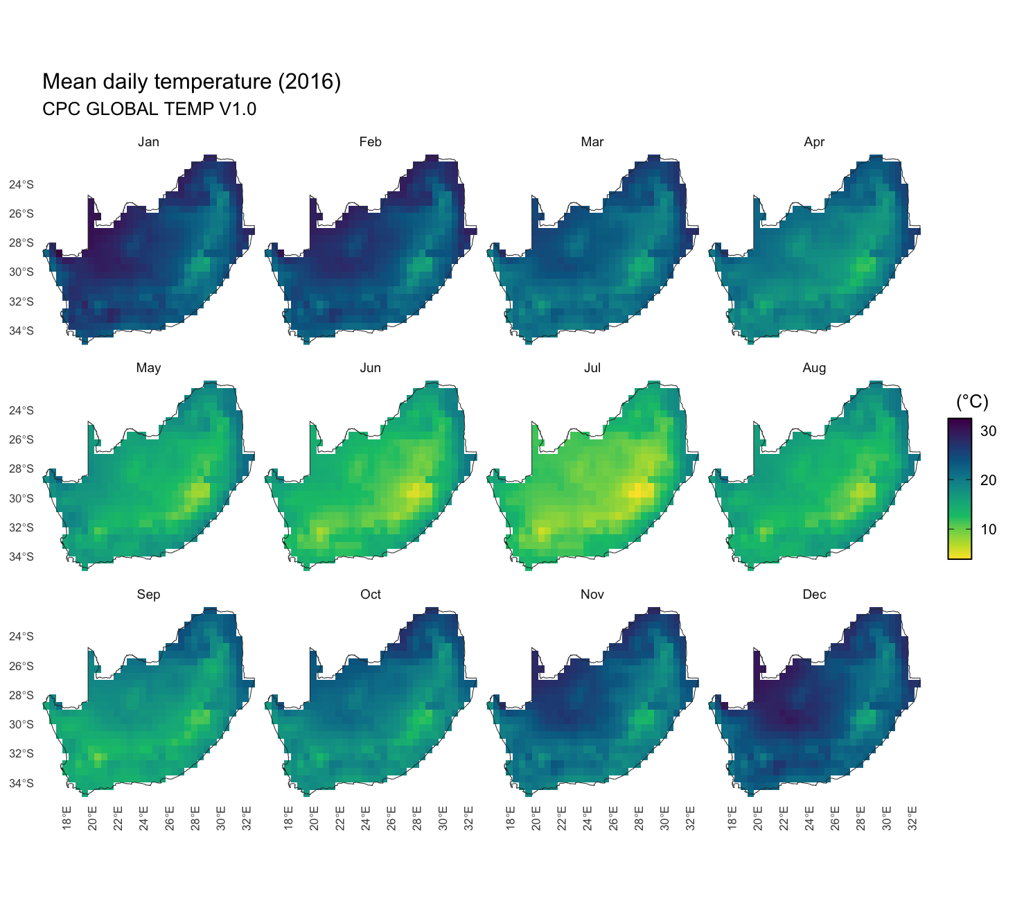
4. Trim (crop) the rainfall and temperature data to the study area as per the shapefile. You are welcome to use NaturalEarth to create a shapefile of the study area, or you can use the shapefile provided in the data files. The shapefile is in the Studyarea subdirectory and is called Studyarea.shp.
5. Create a panelled series of plots showing the mean monthly rainfall (Figure 1) and temperature (Figure 2) for each month of the year.
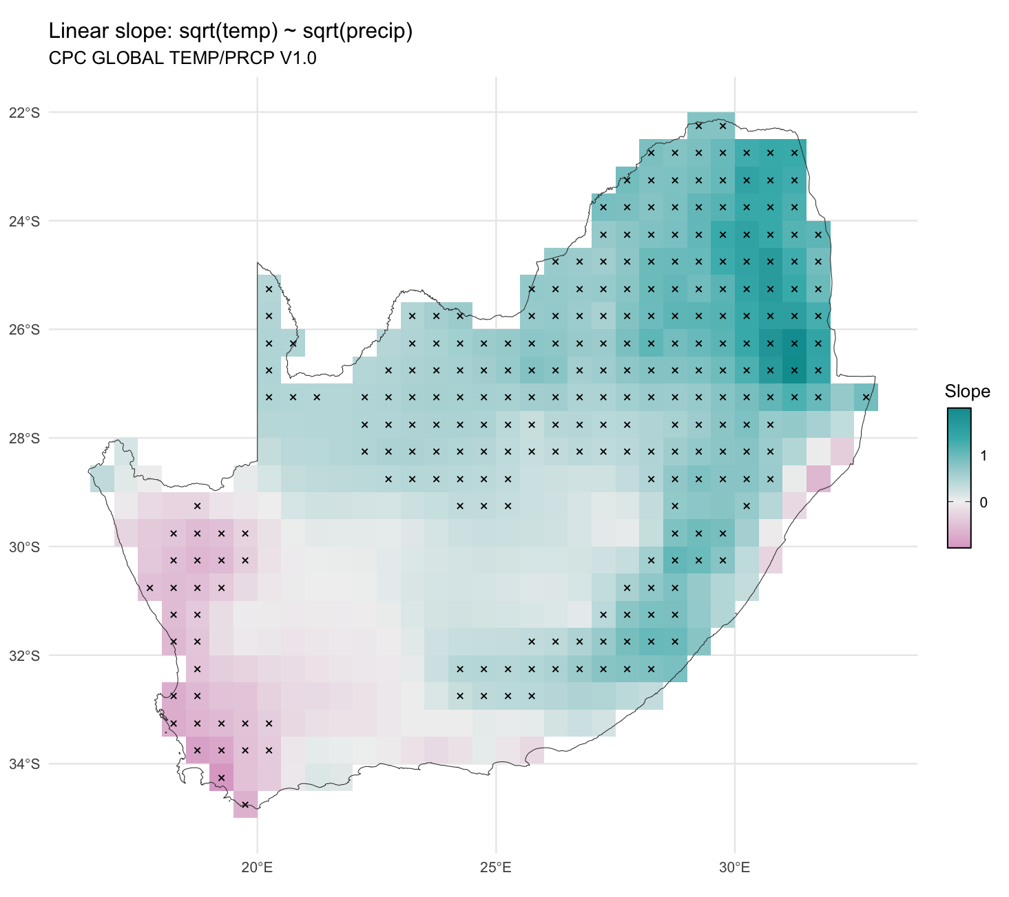
6. Use the square rooted mean monthly surfaces for least square linear regression analysis (i.e. $y=mx+c$) per grid cell, where $x$ represents the square root mean monthly temperature and $y$ represents the square root mean monthly rainfall.
7. Create a new map of the slopes of the per-pixel regressions and indicate which pixels show a trend significantly different from zero based on the the per-pixel p-values (Figure 3).

Hints: The temperature and precipitation data are in NetCDF format. You can use the tidync, terra, stars, or ncdf4 package to read the data. The sf package can be used to manipulate the raster data and shapefiles. I used ddply in the plyr package to fit the linear model to each grid cell. You can also use the purrr and broom packages to do this the tidy way.

In the end, you should aim to recreate the following figures:

Figure 1. Mean monthly temperature over South Africa for the year 2016.

Figure 2. Mean monthly rainfall over South Africa for the year 2016.

Figure 3. Regression coefficient ($r^2$) of $\sqrt{temperature}$ as a function of $\sqrt{precipitation}$ over South Africa for the year 2016. The corsses indicate where the slope is significantly greater than or less than zero.