library(tidyverse)

coughs <- as_tibble(read_csv("AJS_cough_cold_and_flu.csv"))

sales <- coughs %>%
  pivot_longer(2:ncol(coughs), names_to = "province", values_to = "sales") %>%
  mutate(date = as.Date(date),
         sales = as.numeric(sales),
         year = year(date),
         month = month(date),
         week = week(date))

sales_monthly <- sales %>%
  dplyr::mutate(date = floor_date(date, unit = "month")) %>%
  dplyr::group_by(province, date) %>%
  dplyr::summarise(sales = mean(sales, na.rm = TRUE)) %>%
  dplyr::group_by(province) %>%
  dplyr::mutate(anomaly = sales - mean(sales, na.rm = TRUE),
                counter = 1:n()) %>%
  dplyr::group_by(month(date)) %>%
  dplyr::mutate(clim = mean(anomaly)) %>%
  dplyr::ungroup()

ggplot(sales_monthly, aes(x = date, y = anomaly)) +
  geom_line(aes(y = clim), colour = "black", size = 0.9) +
  scale_color_npg() +
  geom_line(aes(colour = province)) +
  theme_linedraw() +
labs(x = "Date", y = "Sales")BCB744 Intro R Example 1
Below is an example of a test or exam question similar to those you may encounter in the BCB744 Intro R course.
This is a practice exercise. While I will not assess your script, I will provide a rubric to guide your self-evaluation. You are expected to complete the task within the allocated time and submit your script to iKamva by the deadline. This allows me to track participation, and I have reason to believe that engagement with these practice tasks correlates with improved performance in the final exam—a hypothesis supported by prior observations.
For your own benefit, I strongly encourage you to work independently. Doing so will ensure that you develop the problem-solving skills necessary for success in the final assessment.
Due date: Monday, 17 February 2025, 17:00.
Part A
The following is an example of a theory-based question. Your task is to provide a written response in paragraph form, explaining the purpose and functionality of the given R script.
You are permitted to use only the R help system to complete this task. Collaboration with others is strictly prohibited.
Your response should include:
- A concise yet thorough explanation of what the script accomplishes as a whole.
- A detailed, line-by-line breakdown of the code, including an explanation of each function used, its arguments, and how they contribute to the script’s overall purpose.
Answer
The provided R script analyses and visualises sales data related to cough, cold, and flu medication across different provinces. It processes raw data, reshapes it into a tidy, long format for better manipulation, calculates monthly sales means, identifies anomalies, and finally generates a time series plot displaying sales anomalies across provinces.
The script uses the tidyverse system of functions, which includes packages such as dplyr, tidyr, and ggplot2, to perform data manipulation and visualisation efficiently.
1library(tidyverse)

2coughs <- as_tibble(read_csv("AJS_cough_cold_and_flu.csv"))

sales <- coughs %>%
3  pivot_longer(2:ncol(coughs), names_to = "province", values_to = "sales") %>%
  mutate(
4    date = as.Date(date),
5    sales = as.numeric(sales),
6    year = year(date),
    month = month(date),
    week = week(date)
  )

sales_monthly <- sales %>%
7  dplyr::mutate(date = floor_date(date, unit = "month")) %>%
  dplyr::group_by(province, date) %>%
8  dplyr::summarise(sales = mean(sales, na.rm = TRUE)) %>%
  dplyr::group_by(province) %>%
  dplyr::mutate(
9    anomaly = sales - mean(sales, na.rm = TRUE),
10    counter = 1:n()
  ) %>%
  dplyr::group_by(month(date)) %>%
11  dplyr::mutate(clim = mean(anomaly)) %>%
  dplyr::ungroup()

12ggplot(sales_monthly, aes(x = date, y = anomaly)) +
13  geom_line(aes(y = clim), colour = "black", size = 0.9) +
14  scale_color_npg() +
15  geom_line(aes(colour = province)) +
16  theme_linedraw() +
17 labs(x = "Date", y = "Sales")- 1
- Load the tidyverse package, which includes functions for data manipulation and visualisation.
- 2
-
Read the CSV file
AJS_cough_cold_and_flu.csvand convert it into a tibble (dataframe) for better handling. - 3
-
Transform the data from wide to long format, creating
provinceandsalescolumns (variables). - 4
-
Convert the
datecolumn to the correct Date format. - 5
-
Ensure the
salescolumn is numeric. - 6
-
Create
year,month, andweekcolumns from thedatefor further analysis. - 7
- Round down dates to the first day of their respective months.
- 8
-
Group data by
provinceandmonth, then calculate the meansalesfor each group. - 9
-
Compute anomalies (
anomaly) by subtracting the meansalesof eachprovincefrom its monthlysales. - 10
-
Add a
countervariable within each province group. - 11
-
Calculate the climatology (
clim) baseline by averaging anomalies for eachmonthacross allprovinces. - 12
-
Create a ggplot object with
dateon the x-axis andanomalyon the y-axis. - 13
- Add a black line representing the climatology baseline to the plot.
- 14
- Apply the Nature Publishing Group (NPG) color palette to the plot.
- 15
-
Add lines representing the
anomalyvalues for eachprovince. - 16
- Use a minimalistic black-and-white theme for the plot.
- 17
- Label the x-axis as “Date” and the y-axis as “Sales”.
Part B
This task requires you to generate a summary table of the class’s task submissions and self-assessments for the BCB744 Intro R course. The workflow has been partially completed—Steps 1 and 2 have been provided, and your task is to write an R script to execute Step 3.
This is an open-book assessment, meaning you are free to use any resources at your disposal. However, collaboration with others is strictly prohibited. If you choose to use an AI tool, you must document the prompts you used to generate the code. These prompts should be included as comments within your script.
Your submission should:
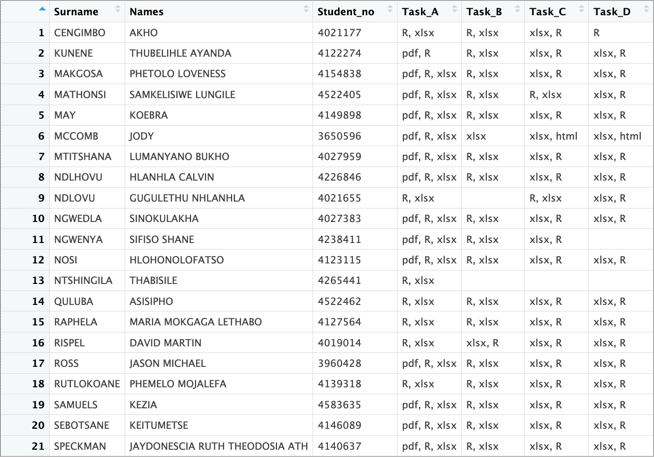
- Ensure that the summary table is structured correctly and clearly presents the required information (see Figure 3).
- Follow best practices in R programming, including clear and well-commented code.
- Be submitted in a format that allows for easy execution and verification of results.
Failure to adhere to these requirements, particularly the documentation of AI-generated assistance, will be taken into account during assessment.
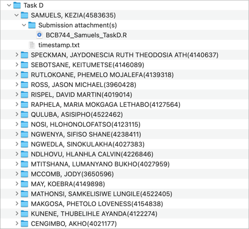
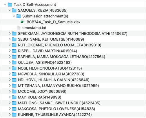
Step 1
I downloaded the submissions from iKamva, and for each task, the directory structure is as follows:
Step 2
Using some Python wizardry, I renamed the files to a standardised format:
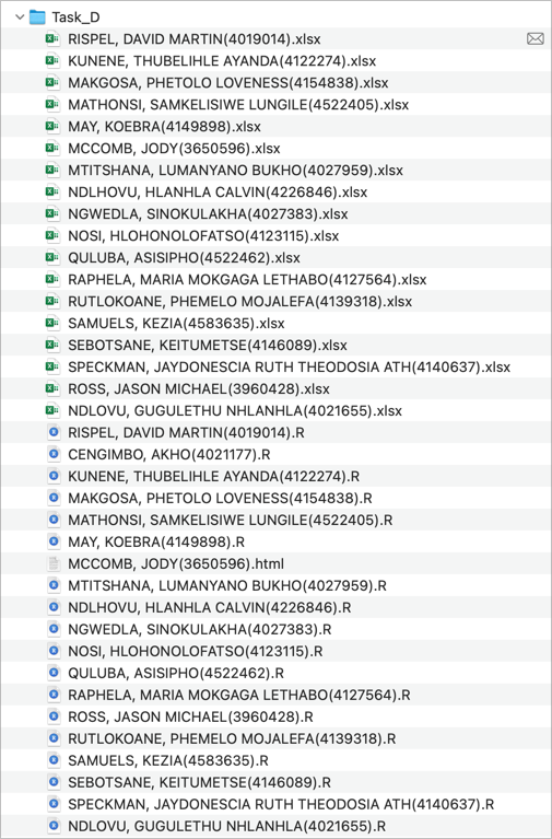
BCB744_Task_D_Samuels.xlsx→SAMUELS, KEZIA(4583635).xlsxBCB744_Samuels_TaskD.R→SAMUELS, KEZIA(4583635).R
The new filenames were derived from the names of the subdirectories within the Task D and Task D Self-Assessment base directories. These names replaced the original basenames (BCB744_Task_D_Samuels and BCB744_Samuels_TaskD), while preserving the file extensions.
Once renamed, my Python script further refined the directory structure by:
- Discarding all subdirectories
- Removing
timestamp.txtfiles - Consolidating all renamed files into a single directory named
Task_D(with equivalent directories for Tasks A–C)
This step is important because the script you will write must extract student names and student numbers directly from the filenames. A consistent naming convention simplifies this process and eliminates unnecessary complexity. This is why I emphasise the importance of structured file-naming practices – adhering to clear conventions minimises errors and streamlines downstream analysis. Fortunately, iKamva enforces a standardised internal naming convention, ensuring that student submissions follow a predictable format. Thus, even if user-assigned filenames vary, they can be corrected by replacing them with the systematically structured subdirectory names.
After applying this renaming workflow, the resulting directory structure appears as follows:
To facilitate the next step, I saved the directory contents as text files:
- Task_A.txt
- Task_B.txt
- Task_C.txt
- Task_D.txt
Each of these .txt files lists both .R and .xlsx files within their respective task directories.
Next Steps
You will not have access to the original files – only the .txt listings. These text files can be downloaded here, and you will use them to complete Step 3.
Step 3
Using R, you will process the provided .txt files as input and generate a summary table (Figure 3) detailing all student submissions for each task. Your script should systematically extract relevant information from the filenames, organise the data, and compile a structured summary.
Once complete, save the resulting table as a .csv file to ensure easy review and further analysis.
Answer
library(tidyverse)

base_dir <- "/Users/ajsmit/Library/CloudStorage/Dropbox/BCB744"

Task_A <- read_csv(paste0(base_dir, "/Task_A.txt"),
                   show_col_types = FALSE, col_names = FALSE)
Task_B <- read_csv(paste0(base_dir, "/Task_B.txt"),
                   show_col_types = FALSE, col_names = FALSE)
Task_C <- read_csv(paste0(base_dir, "/Task_C.txt"),
                   show_col_types = FALSE, col_names = FALSE)
Task_D <- read_csv(paste0(base_dir, "/Task_D.txt"),
                   show_col_types = FALSE, col_names = FALSE)

# Create a list of the tasks
Task_list <- list(Task_A = Task_A,
                  Task_B = Task_B,
                  Task_C = Task_C,
                  Task_D = Task_D)

# Create a long dataframe
Task_long <- bind_rows(Task_list, .id = "Task")

# Rename columns 2 and 3 as 'Surname' and 'Name', respectively
Task_long <- Task_long %>%
  rename(Surname = X1, Name = X2)

# Split the content of the 'Name' column into three parts:
# 1. 'Names' before the opening brace '('
# 2. 'Student_no' between the opening and closing braces
# 3. 'File_ext' after the period '.'
Task_long <- Task_long %>%
  separate(Name, into = c("Names", "Student_no", "File_ext"),
           sep = "[\\(\\)]")

# For the 'File_ext' column, remove the period '.'
Task_long$File_ext <- gsub("\\.", "", Task_long$File_ext)

# For each 'Sstudent_no' (which corresponds to a student):
# 1. Create four new columns ('Task_A', "task_B', etc.) based on the
# content of the 'Task' column
# 2. Populate the new columns with a concatenation of the file extensions
# named in the 'File_ext' column
# (e.g. 'R', 'xlsx', etc., with each file extension separated by a comma)
Task_wide <- Task_long %>%
  pivot_wider(names_from = Task, values_from = File_ext)

# List of columns to process
cols_to_process <- c("Task_A", "Task_B", "Task_C", "Task_D")

# Apply function to each column and replace its content
Task_wide[cols_to_process] <- lapply(Task_wide[cols_to_process],
                                     function(col)
                                       sapply(col, function(x)
                                         paste(x, collapse = ", ")))
Reuse
Citation
@online{smit,_a._j.,
  author = {Smit, A. J.,},
  title = {BCB744 {Intro} {R} {Example} 1},
  url = {http://tangledbank.netlify.app/assessments/examples/BCB744_Intro_R_Example_1.html},
  langid = {en}
}


