11. Tidy Data

“Order and simplification are the first steps toward the mastery of a subject.”
— Thomas Mann
“Get your facts first, and then you can distort them as much as you please.”
— Mark Twain
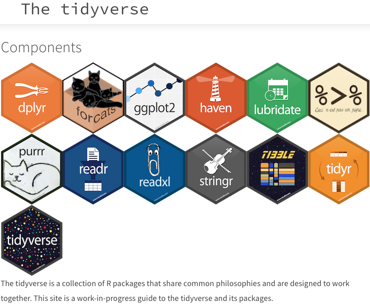
The Tidyverse is a collection of R packages designed for data manipulation, exploration, and visualisation. It is based on a philosophy of ‘tidy data,’ which is a standardised way of organising data. The purpose of these packages is to make working with data more efficient. The core Tidyverse packages were created by Hadley Wickham, but over the last few years other individuals have added some packages to the collective, which has significantly expanded our data analytical capabilities through improved ease of use and efficiency. All packages that are built on tidy principles provide the use of a consistent set of tools across a wide range of data analysis tasks. The core Tidyverse packages can be loaded collectively by calling the tidyverse package, as we have seen throughout this workshop. The packages making up the Tidyverse are shown in Figure 1.
Properties of tidy data
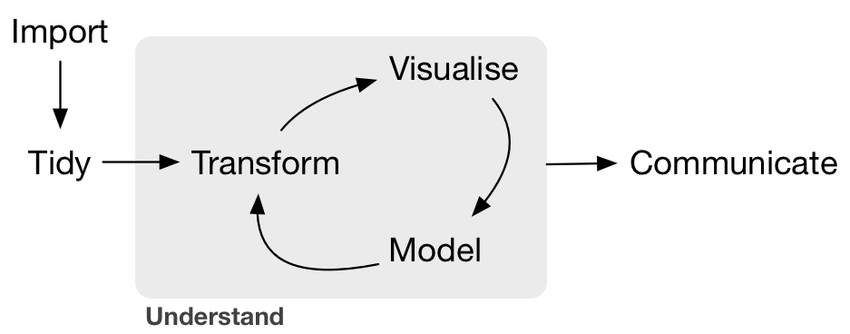
As you may see in Figure 2, the tidying of ones data should be the second step in any workflow, after loading the data.
But what exactly are tidy data? It is not just a a buzz word, there is a real definition. In three parts, to be exact. Taken from Hadley Wickham’s R for Data Science:
Consider this example of tidy data:
R> # A tibble: 10 × 5
R>    region site                Ind measurement       value
R>    <chr>  <chr>             <dbl> <chr>             <dbl>
R>  1 WC     Kommetjie            11 stipe_mass         4.2
R>  2 WC     Kommetjie            11 stipe_length     176
R>  3 WC     Kommetjie            11 stipe_diameter    76
R>  4 WC     Kommetjie            11 digits             8
R>  5 WC     Kommetjie            11 thallus_mass    6500
R>  6 WC     Kommetjie            11 total_length     354
R>  7 FB     Bordjiestif North     1 blade_weight       1.75
R>  8 FB     Bordjiestif North     1 blade_length     145
R>  9 FB     Bordjiestif North     1 blade_thickness    1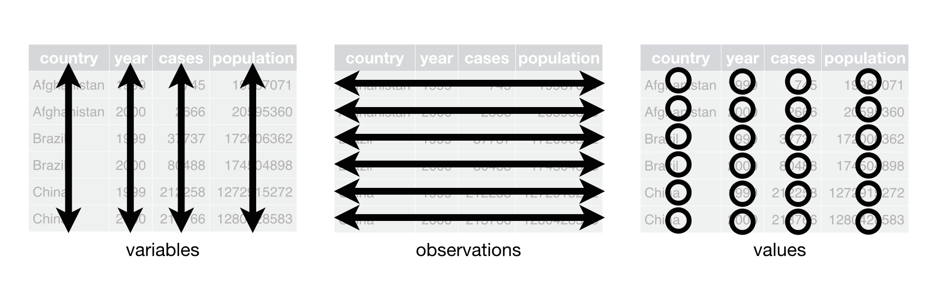
R> 10 FB Bordjiestif North 1 stipe_mass 0.75- Each variable must have its own column. Some of the variables tell us about the measurements (the
regionwhere thesitewas located, the replicate number (ind) of the plants sampled, and the nature of themeasurementtaken), and one variable gives thevalueof the measurement. - Each measurement must have its own row—the value of each of the things measured must be in its own row; for example, in the Laminaria data the measured things include
blade_length,blade_weight, etc., and they can all be captured in one column named, for example,measurement. - Each
valuemust have its own cell—each of the things that is known and measured must be in its own cell.
The core principle of tidy data is represented graphically in Figure 3). One will generally satisfy these three rules simply by never putting more than one dataset in a file, and never putting more (or less) than one variable in the same column. We will go over this several more times today so do not fret if those guidelines are not immediately clear.
Grammar of data manipulation The Tidyverse provides a set of functions and tools for data manipulation that can be combined in a way that is similar to a grammar. This makes it easy to write complex data manipulation tasks, and also makes it easier to read and understand code written by others.
Consistent style The Tidyverse provides a consistent style for functions and data structures, making it easier to work with multiple packages within the Tidyverse, as well as with other R packages.
Interoperability The Tidyverse is designed to work seamlessly with other R packages, so that data can be easily moved between different analysis pipelines.
Different ways to be untidy
In order to illustrate the meaning of this three part definition, you are going to learn how to manipulate a non-tidy dataset into a tidy one. To do so you will need to learn a few new, very useful functions. Load your demo dataset to get started. This snippet from the SACTN dataset contains only data for 2008-2009 for three time series, with some notable (untidy) changes. The purpose of the following exercises is not only to show how to tidy data, but to also illustrate that these steps may be done more quickly in R than MS Excel, allowing for your raw data to remain exactly how they were collected, with all of the manipulations performed on them documented in an R script. This is a centrally important part of reproducible research.
With the SACTN_mangled.RData data loaded, have a peek at them. You will first see that you’ve loaded not one, but five different objects into our environment pane in the top right of our RStudio window. These all contain the exact same data in different states of disrepair. As you may have guessed, some of these datasets will be easier to use than others.
Start off by looking at SACTN1. If these data look just like all of the other SACTN data we’ve used thus far that’s because they are. These are how tidy data should look. No surprises. In fact, because these data are already tidy it is very straightforward to use them for whatever purposes we may want. Making a time series plot, for example.

Long and wide formatted data
Before tidy became the adjective used to describe neatly formatted data, people used to say long. This is because well organised dataframes tend to always be longer than they are wide (with the exception of species assemblage data). The opposite of long data are wide data. If you ever find a dataset that is wider than it is long then this is probably because the person that created them saved one variable across many columns.
It may seem odd that so much effort is being spent on something so straightforward as tidy data. Surely this is too obvious to devote an entire day of work to it? Unfortunately not. As you go out into the wild world of ‘real life data’, you’ll discover that very few datasets (especially those collected by hand) are tidy. Rather they are plagued by any number of issues. The first step then for tidying up the data is to have a look at them and separate the observations that were made/recorded (the ‘measurements’) from the variables within those observations. You also need to know something about how or where the data were collected, or what they represent—this is information about the data, i.e. some meta-data.
pivot_longer()
The R function pivot_longer() is a useful tool for transforming data from wide to long format. It belongs to the tidyr package (loaded with tidyverse) and allows you to reshape your dataframe by gathering multiple columns into key-value pairs. Specifically, pivot_longer() takes in a dataframe and allows you to select a set of columns that you would like to pivot into longer format, while specifying the names of the key and value columns that you want to create. The resulting data frame will have a new row for each unique combination of key and value pairs. This function is particularly useful when you need to reshape your data in order to carry out certain analyses or visualisations.
Have a look now at SACTN2 for an example of what wide data look like, and how to fix it.
In SACTN2 you can see that the src column has been removed and that the temperatures are placed in columns that denote the collecting source. This may at first seem like a reasonable way to organise these data, but it is not tidy because the collecting source is one variable, and so should not take up more than one column (i.e. there are multiple observations per row). You need to gather these source columns together into one column so that the seperate measurements (observations) can conform to the one observation per row rule. You do this by telling pivot_longer() the names of the columns you want to squish together. You then tell it the name of the key (names_to) column. This is the column that will contain all of the old column names we are gathering. In this case you may call it source. The last piece of this puzzle is the value (values_to) column. This is where you decide what the name of the column will be for measurements you are gathering up. In this case you may name it temperature, because you are gathering up the temperature values that were incorrectly spread out by the source of the measurements.
- Using the tidy data (
SACTN2_tidy) and untidy data (SACTN2), create line graphs, one for each of DEA, SAWS, and KZNSB, showing a time series of temperature. ForSACTN2_tidyandSACTN2, make sure you have a column of three figures (ncol = 1). Use the fewest number of lines of code possible.
You should end up with two graphs, each with three panels.
Task G must be submitted together with the Summative End-of-Intro-R Task, the final assignment in the Intro R portion of BCB744.
pivot_wider()
The function pivot_wider() is a tool for transforming data from long to wide format. It is the counterpart to the pivot_longer() function. pivot_wider() allows you to take a set of columns containing key-value pairs and convert them into a wider format, where each unique key value becomes a separate column in the resulting data frame. You can also specify a set of value columns that you want to spread across the new columns created by the key values. With pivot_wider(), you can quickly transform your data from long format into a more intuitive, wide format that is easier to work with in some applications.
Should your data be too long for a particular application (typically a non-Tidyverse application) or your liking, meaning when individual observations are spread across multiple rows, you will need to use pivot_wider() to rectify the situation. This is generally the case when you have two or more variables stored within the same column, as you will see in SACTN3. This is not terribly common as it would require someone to put quite a bit of time into making a dataframe this way. But never say never. To spread data to become wider, you first tell R what the name of the column is that contains more than one variable, in this case the var column. You then tell R what the name of the column is that contains the values that need to be spread, in this case the val column.
Separating and uniting
You’ve now seen how to make our dataframes longer or wider depending on their tidiness. Now you will look at how to manage our columns when they contain more (or less) than one variable, but the overall dataframe does not need to be made wider or longer. This is generally the case when one has a column with two variables, or two or more variables are spread out across multiple columns, but there is still only one observation per row. Here are some examples to make this clearer.
Separate
Looking at SACTN4a, you see that you no longer have a site and src column. Rather these have been replaced by an index column. This is an efficient way to store these data, but it is not tidy because the site and source of each observation have now been combined into one column (variable). Remember, tidy data calls for each of the things known about the data to be its own variable. To re-create site and src columns, you must separate the index column. There are two options: separate_wider_delim() and separate_wider_position(). What does each do? First you give R the name of the column you want to separate, in this case index. Next you specify what the names of the new columns will be. Remember that because we are creating new column names you feed these into R within inverted commas. Lastly, you should tell R where to separate the index column. If you look at the data you will see that the values you want to split up are separated with / (including a space), so that is what you need to tell R.
Separating dates using mutate()
Although the date column represents an example of a date date type or class (a kind of data in its own right), you might also want to split this column into its constituent parts, i.e. create separate columns for day, month, and year. In this case you can spread these components of the date vector into three columns using the mutate() function and some functions in the lubridate package (part of the tidyverse).
Note that when the date is split into component parts the data are no longer tidy (see below).
Unite
It is not uncommon that field/lab instruments split values across multiple columns while they are making recordings. You might sometimes see this with date values where the year, month, and day values are given in different columns. There are uses for the data in this way, though it is not terribly tidy. You usually want the date of any observation to be shown in just one column. If you look at SACTN4b you will see that there is a year, month, and day column. To unite() them you must first tell R what you want the united column to be labelled, in this case you will use date. You then list the columns to be united; here this is year, month, and day. Lastly, decide if you want the united values to have a separator between them. The standard separator for date values is ‘-’.
Joining
Now you will see the process for joining two different dataframes. Remember that one of the rules of tidy data is that only one complete dataset is saved per dataframe. This rule then is violated not only when additional data are stored where they don’t belong, but also when necessary data are saved elsewhere. Looking back at SACTN4a and SACTN4b, you will see that they are each missing different columns. Were you to join() these dataframes together they would complete each other. The tidyverse provides several methods of doing this, but you will see in action the most common technique to use. The function left_join() is so named because it joins two or more dataframes together based on the matching of columns from the left to the right. It combines values together where it sees that they match up, and adds new rows and columns where they do not.
R> Joining with `by = join_by(site, src, date)`As you see above, if you let left_join() do it’s thing it will make a plan for and find the common columns and match up the values and observations for you as best it can. It then returns a message letting you know what it’s done. That is a pleasant convenience, but you most likely want to exert more control over this process than that. In order to specify the columns to be used for joining you must add one more argument to left_join(). The by argument must be fed a list of column names in inverted commas if you want to specify how to join our dataframes. Note that when you run this it does not produce a message as you have provided enough explicit information that the function is no longer needing to ‘think’ for itself.
There are also other kinds of joins: see for example also inner_join, right_join, full_join, semi-join, nest_join, and anti_join in the dplyr package contained within tidyverse.
But why though?
At this point you may be wondering what the point of all of this is. Sure it’s all well and good to see how to tidy your data in R, but couldn’t this be done more quickly and easily in MS Excel? Perhaps, yes, with a small dataset. But remember, (for many) the main reason you are learning R is to ensure that you are performing reproducible research. This means that every step in our workflow must be documented. And you accomplish this by writing R scripts, and part of the purpose of these scripts is to ensure that you capture all the steps taken to get the raw data into a neat and tidy format that can unambiguously be read into R in the format that will quicky get you up and running with your analyses and visualisations.
Session info
Reuse
Citation
@online{j._smit2021,
  author = {J. Smit, Albertus},
  title = {11. {Tidy} {Data}},
  date = {2021-01-01},
  url = {http://tangledbank.netlify.app/BCB744/intro_r/11-tidy.html},
  langid = {en}
}