Lecture 2b: Metrics of Environmental Distance & Species Diversity

This material must be reviewed by BCB743 students in Week 1 of Quantitative Ecology.
Quantifying Diversity
When we talk about ‘biodiversity,’ we typically refer to the variety of life in a given area or ecosystem. This encompasses species diversity, genetic diversity within species, and the diversity of ecosystems or habitats. To quantify biodiversity, we use metrics that capture various aspects, including:
- The variability and characteristics of the environment.
- The species present in a given area (species lists).
- The relative abundance of each of the species.
- The spatial distribution of species across different habitats or ecosystems.
In this lecture, we will explore some of the most common metrics used to quantify biodiversity. We’ll delve into the concepts of species richness, evenness, and diversity, and how these metrics can be applied to compare different habitats or ecosystems.
Biodiversity metrics can be broadly categorised into three groups based on the type of information they provide:
- Biodiversity metrics (
- Diversity indices (e.g., Shannon’s Entropy, Gini Index, Herfindahl-Hirschman Index (HHI)).
- Distance measures (e.g., Euclidean, Manhattan) and Dissimilarity indices (e.g., Bray-Curtis, Jaccard, Sørensen).
The first two categories—biodiversity metrics and diversity indices—offer simplified representations of biodiversity through synthetic metrics or indices. In contrast, distance measures and dissimilarity indices provide more nuanced and detailed insights by exposing the full multivariate information within our datasets. This allows for a deeper examination of the processes driving community formation and the resulting structures that describe biodiversity patterns across landscapes.
Biodiversity Metrics
Alpha diversity quantifies the diversity of species within a specific, localised area or community. This could be a site, plot, quadrat, a field, or any other small unit of (typically) replication in the study. This measure provides information about the ecological structure and complexity of a given habitat at a fine scale.
There are several ways to represent
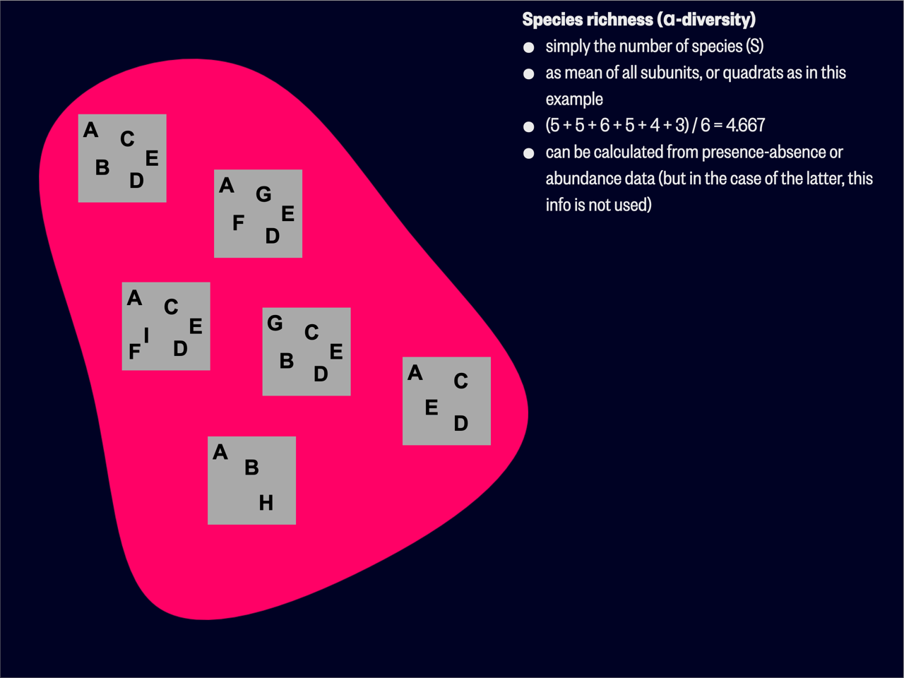
Species richness is easy to understand and implement, but it doesn’t account for the relative abundance of each species within the community. To address this limitation we make use of univariate indices. Shannon’s H’ (Shannon’s Diversity Index) and Simpson’s
Choosing Shannon’s or Simpson’s is a bit controversial and it often depends on who is using it. According to Jari Oksanen, author of the vegan package in R, the choice between Shannon’s and Simpson’s index is a matter of personal preference. He writes:
Better stories can be told about Simpson’s index than about Shannon’s index, and still grander narratives about rarefaction (Hurlbert 1971). However, these indices are all very closely related (Hill 1973), and there is no reason to despise one more than others (but if you are a graduate student, don’t drag me in, but obey your Professor’s orders). In particular, the exponent of the Shannon index is linearly related to inverse Simpson (Hill 1973) although the former may be more sensitive to rare species.
Both Shannon’s H’ or Simpson’s
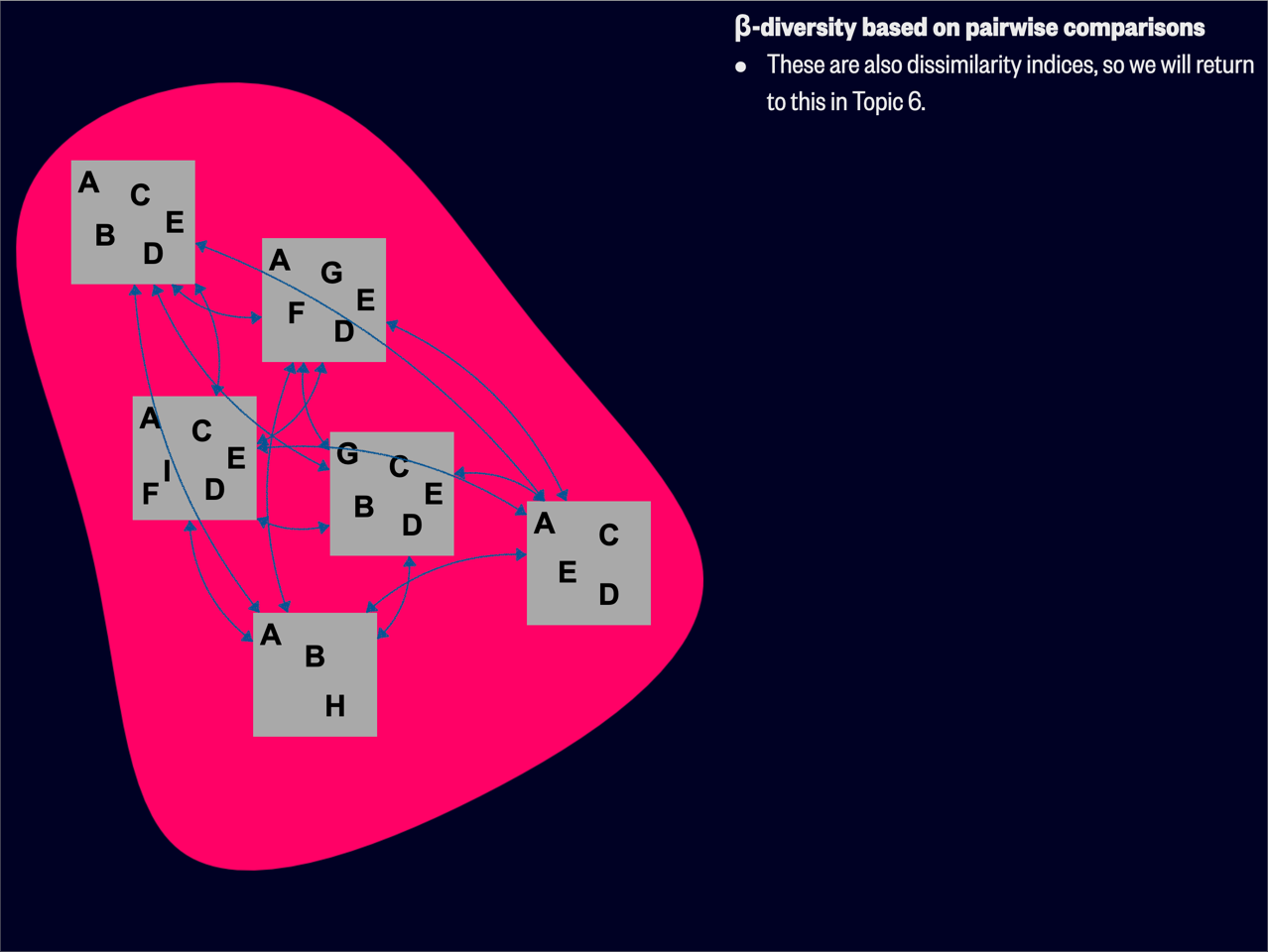
A related concept of diversity is one that considers the variation between sites (Figure 2). This is known as
Whittaker’s initial idea was that of true
where
Another approach is absolute species turnover, which is a measure of the total amount of species change between communities or along environmental gradients. It can be calculated in various ways, but one common approach is to use the Whittaker’s
where
This measure of turnover ranges from 0 (when all communities have identical species composition) to a maximum value that depends on the number of communities being compared. It provides a quantitative measure of how much species composition changes across communities or sites.
Contemporary views of
Process 1: If a region comprises the species A, B, C, …, M (i.e. beta() in the R package BAT calls this form of
Process 2: Consider again species A, B, C, …, M. Now we have a quadrat with species A, B, C, D, G, H (beta() in the R package BAT calls this form of
The above two examples show that
We express
According to Nekola and White (1999) on p. 868, there are two causes of ecological distance decay. ‘Ecological’ is key to the first cause—it is environmental filtering results in a decrease in similarity as the distance between sites increases. We sometimes call this the niche difference model. Such patterns are typically visible along steep environmental gradients such as elevation slopes (mountains), latitude, or depth in the ocean, to name only three. It is also the dominant mechanism underlying island biogeography.
The second cause of distance decay sensu Nekola and White (1999) involves aspects of the spatial configuration, context of the habitats, and some temporal considerations. Here, the evolutionary differences between species—specifically around those traits that affect their ability to disperse—are more at play and are the primary influences of distance decay rates that might vary between species. Let us first consider some properties of a hypothetical homogeneous landscape. The landscape creates some impediment (resistance) to the propagation of some species (hypothetically species A, B, and C) across its surface, but which are less effective in impeding others (D, E, and F). For argument’s sake, all species (A, …, F) share similar environmental tolerances to the prevailing environmental conditions, so one can argue that the niche difference model (environmental filtering) does not explain distributional patterns. Given a particular founding or disturbance event, species D, E, and F will, in a relatively shorter period, be able to become evenly distributed (relatively similar abundances everywhere) across this landscape. However, the less vagile (in terms of dispersal ability), species A, B, and C will develop a steeper gradient of decreasing species abundances away from the founding populations (resulting from, for example, adaptive radiation). They will require more time to become homogeneously dispersed across the landscape. In this regard, historical events set up striking distributional patterns that can be mistaken for gradients, which exist because insufficient time has passed to ensure complete dispersal. Studying the influence of such past events is called ‘historical biogeography.’ In reality, landscapes are seldom homogeneous in their spatial template (e.g. there are hills and valleys), and variable dispersal mechanisms and abilities will interact with this heterogeneous landscape to form interesting patterns of communities. The ecologist will have an exciting time figuring out the relative importance of actual gradients vs those that result from evolved traits that affect their dispersal ability and interact with the environment. I have not said anything about ‘neutral theories’ (but which are seen in the
While
Diversity Indices
A diversity index is a metric that quantifies species diversity within a community. While species richness simply refers to the number of species present, diversity indices also consider the relative abundances of these species. For instance, consider two communities: community A comprises 10 individuals of each of 10 species (totalling 100 individuals) and community B has 9 species with 1 individual each, and a 10th species with 91 individuals (also totalling 100 individuals). Which community is more diverse? To address this, diversity indices incorporate both richness and evenness information and provides a more comprehensive assessment of diversity than species richness alone.
Margalef’s Index
Margalef’s Index is a simple measure of species richness that accounts for the number of species in a community and the total number of individuals. The formula for Margalef’s Index is:
where
Shannon’s Entropy
Shannon’s Entropy, or Shannon’s H’, comes out of the field of information theory and was developed by Claude Shannon. It measures the uncertainty or diversity within a system. It is a general measure of information content and is applicable to a variety of data types beyond species diversity, such as genetic diversity, linguistic diversity, or even the distribution of different types of land use in a landscape. The formula for Shannon’s H’ is as used by ecologists is:
where
Simpson’s Indices
Simpson’s Indices are a group of related diversity measures developed by Edward H. Simpson. These indices focus on the dominance or evenness of species in a community, giving more weight to common species and being less sensitive to species richness compared to Shannon’s H’.
Simpson’s Dominance Index
Simpson’s Dominance Index (
where
Simpson’s Diversity Index
To make the index more intuitive we prefer to use Simpson’s Diversity Index, which is calculated as:
This form ensures that the index increases with increasing diversity. Values range from 0 to 1, with higher values indicating higher diversity.
Simpson’s Reciprocal Index
Another common form is Simpson’s Reciprocal Index, calculated as:
This index starts with a value of 1 as the lower limit, representing a community containing only one species. The upper limit is the number of species in the sample (S). Higher values indicate greater diversity.
Simpson’s Indices are less sensitive to species richness and more sensitive to evenness compared to Shannon’s Entropy. They are useful when you want to give more weight to common species in your diversity assessment.
Gini Index
The Gini Index, or Gini Coefficient, should be fimiliar to all South Africans—South Africa is infamous for having the highest Gini Coefficient in the world. The Gini Index is a measure of inequality within a distribution, and is typically used in economics to assess income or wealth inequality. Since its purpose is to evaluate disparity, it is also suited to ecological systems because, here too, the distribution in abundance differs among species. The formula for the Gini Index is:
where
Herfindahl-Hirschman Index (HHI)
The Herfindahl-Hirschman Index (HHI) is a measure of market concentration commonly used in economics to assess the level of competition within an industry. It is calculated as the sum of the squares of the market shares of all firms in the market. Ecologists sometimes use the HHI to assess species dominance or the concentration of individuals within species. The formula for HHI is:
where
Here’s a corrected and improved version of the text:
Ecological Resemblance
Resemblance matrices are mathematical representations used to quantify the similarity or dissimilarity between pairs of samples, communities, or ecological sampling units based on various criteria such as species composition, abundance, functional traits, phylogenetic relatedness, or environmental properties. Well-structured raw data about species composition typically come in the form of a table with rows representing sites or samples, and columns representing species. Similarly, data about environmental variables are structured as a table with rows representing sites or samples, and columns representing environmental variables.
The diagram below (Figure 4) summarises the species and environmental data tables, and what we can do with them. These tables are the starting points of many additional analyses, and we will explore some of these deeper insights later in this module.
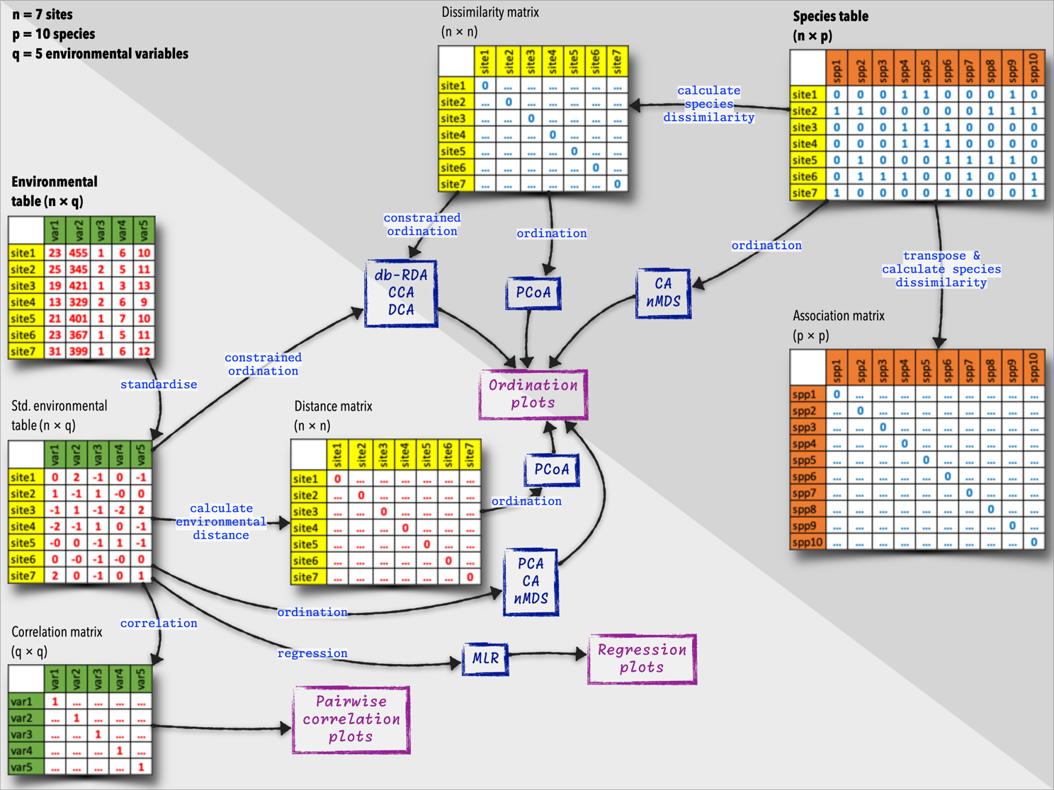
Although we often use the terms ‘matrix’ and ‘table’ interchangeably, in this book I use matrix to refer to a mathematical object with rows and columns and with the cell content derived from calculations of distances and dissimilarities. In these situations they tend to be square and symmetrical. I then use the term table to refer to a more general data structure, also with rows and columns, but here representing samples or sites (as rows) and columns representing species or environmental variables. My use of ‘table’ generally refers to the raw data we use as a starting point for our calculations (including of the matrices).
This is my notations and authors such as Borcard et al. (2011), David Zelený, and Michael Palmer may not make this distinction and use both terms to refer to a rectangular data structure.
When the focus is on comparing sites (i.e., the information about objects in the rows of site × species or site × environment tables) based on their species composition or environmental characteristics, we call this type of analysis an R-mode analysis. Such resemblance matrices typically manifest as square matrices, with rows and columns representing the samples or units being compared.
Other cases of square resemblance matrices include: i) Species-by-species matrices (association matrices), where both rows and columns represent species, and the values in the matrix represent the association between each pair of species. ii) Environmental-by-environmental matrices (correlation matrices), where both rows and columns represent environmental variables, and the values in the matrix represent the correlation between each pair of variables. In these cases, the focus falls onto the information initially contained in the columns (species or descriptors) of the sites × species table or the sites × environmental variables table. This is called a Q-mode analysis.
Environmental resemblance matrices, or environmental distance matrices, are used to quantify the similarity between pairs of sites based on their environmental variables. They can also be used in more advanced analyses, such as various kinds of ordinations and clustering. These matrices have zeros down the diagonal, as the distance between a site and itself is zero. The subdiagonal values are typically the same as the superdiagonal values, as the dissimilarity between samples
In species dissimilarity matrices (species resemblance matrices), the values represent the degree of dissimilarity between each pair of samples. Dissimilarity matrices are characterised by a diagonal filled with zeros, because the dissimilarity between a sample and itself is zero. The off-diagonal values represent the dissimilarity between pairs of samples, with higher values indicating greater dissimilarity. They are also symmetrical for the same reasons given for the environmental matrices. Species dissimilarity matrices are used in various multivariate analyses, such as cluster analysis, ordination, and diversity partitioning.
Legendre and Legendre (2012) provide a full chapter (Chapter 7) on ecological resemblance, including an in-depth look at the various kinds of ‘association coefficients,’ which is what we will cover next. The next two sub-sections will thus introduce a few frequently used association coefficients to study species dissimilarity and environmental distances across the landscape.
Environmental Distance
Sometimes we need to quantify the environmental similarities or differences between sampling sites, such as plots, quadrats, or transects. This is typically achieved through the use of distance matrices (one kind of resemblance matrix), which provide an overall view of how all the sites relate to one another. These matrices are derived from data tables containing information on environmental variables (sites in rows and variables in columns).
There are several kinds of distance metrics available for use with environmental data. Regardless of which index one chooses, the resulting matrix provides pairwise differences (or distances) or similarities in a metric that relates to the ecological distance between all sites (and which might also link to their community composition, which is the thing we are trying to determine). Such pairwise matrices are foundational for various multivariate analyses and can reveal patterns in ecological data that might not be apparent from raw measurements of individual variables alone.
Euclidean distance is in my experience the commonly used in spatial analysis. It defined as the straight-line distance between two points in Euclidean space. In its simplest form, it applies to a planar area such as a graph with
Mathematically, Euclidean distance is calculated using the Pythagorean theorem. This method squares the differences between coordinates, which means that single large differences become disproportionately important in the final distance calculation. While this property makes Euclidean distance useful for environmental data, where it effectively calculates the ‘straight-line distance’ between two points in multidimensional space (with each dimension representing an environmental variable), it is ill suited to species data.
The Euclidean distance between two points
where
Other distance metrics are the Mahalanobis Distance, Manhattan Distance, Canberra Distance, Gower Distance, and Bray-Curtis Dissimilarity. I’ll not discuss them here and you can refer to Chapter 3 in the book by Borcard et al. (2011) for more information. Additionally, vegan’s vegdist() function does a very good job of providing a wide range of distance metrics and you can find a discussion of many of them in the function’s help file, which you can access as ?vegan::vegdist.
Species Dissimilarities
Ecological similarity between sites is fundamentally tied to their species composition, which is a function of both species richness and abundance. Sites that share similar species compositions are considered ecologically similar and exhibit a low dissimilarity metric. The factors influencing this similarity are complex and influenced by many properties of the environment and processes operating there.
As we have already seen, the degree of similarity between sites can be attributed to measurable environmental differences (i.e. hopefully captured in the environmental distance matrices we saw above) that directly influence species composition. These might include variables like soil type, climate, or topography. However, similarity can also be affected by unmeasured, often overlooked influences that are not immediately apparent or easily quantifiable. Additionally, some degree of variation may simply be attributed to ecological ‘noise’—random fluctuations or stochastic events that affect species distributions.
It is our role to disentangle these various influences and determine the primary drivers of similarity or dissimilarity among sites. To aid in this analysis, we use a class of matrices known as dissimilarity matrices (a type of resemblance matrix). These matrices quantify the dissimilarity between sites based on their species composition.
Various indices have been developed to compare the composition of different groups or communities. These diversity indices quantify how different or similar groups are based on their attributes, primarily species richness and/or relative abundances. While the simplest application is to compare the species composition of two sites, these indices can be extended to compare multiple groups or communities. They are core to the study of β-diversity, which examines the variation in species composition among sites within a geographic area.
I’ll present the Bray-Curtis dissimilarity as an example, which is a widely-used metric for comparing species composition between two sites. For abundance data, it is calculated as follows:
where
For presence-absence data, the Bray-Curtis dissimilarity simplifies to:
where
The Bray-Curtis dissimilarity ranges from 0 (indicating identical species compositions) to 1 (indicating completely different compositions). This metric can be used to construct dissimilarity matrices for multivariate analyses, where each cell in the matrix represents the ecological distance between a pair of sites based on their species composition.
In practice, these dissimilarity indices and distances can be calculated using the vegan R package’s vegdist() function. Refer to ?vegan::vegdist for information and a deeper look.
Common dissimilarities suited to presence-absence data are the Jaccard Dissimilarity, Sørensen-Dice index, and Ochiai index. For abundance data, we have already seen the Bray-Curtis dissimilarity, but you also have the Morisita-Horn index, which is also commonly used. The Raup-Crick index is used to compare the dissimilarity between two groups to the expected dissimilarity between two random groups, whilst the Chao-Jaccard and Chao-Sørensen indices are probabilistic versions of the Jaccard and Sørensen indices that account for unseen shared species.
References
Reuse
Citation
@online{smit,_a._j.2024,
  author = {Smit, A. J.,},
  title = {Lecture 2b: {Metrics} of {Environmental} {Distance} \&
    {Species} {Diversity}},
  date = {2024-07-22},
  url = {http://tangledbank.netlify.app/BDC334/L02b-biodiversity.html},
  langid = {en}
}