Lecture 3: Species Distribution Patterns

Author

Affiliation

Albertus J. Smit

University of the Western Cape

BCB743

This material must be reviewed by BCB743 students in Week 1 of Quantitative Ecology.

This Lecture is Accompanied by the Following Lab

• Lab 4. Species Distribution Patterns

Reading Required For This Lab

• Gotelli and Chao (2013)
• Matthews and Whittaker (2015)
• Shade et al. (2018)

Univariate diversity measures such as Simpson and Shannon diversity have already been prepared from species tables, and we have also calculated measures of \(\beta\)-diversity that looked at pairwise comparisons and offered insight into community structure across a landscape and hinted at the processes that might have resulted in these structures. These ways of expressing biodiversity only gets us so far in understanding the structure of communities. A much deeper insight into the processes responsible for community formation can be obtained by looking at how the species patterns are distributed across sites. This is the focus of this lecture.

Let’s shine the spotlight to additional views on ecological structures and the ecological processes that structure the communities—sometimes we will see reference to ‘community or species formation processes’ to offer mechanistic views on how species come to be arranged into communities (the aforementioned turnover and nestedness-resultant \(\beta\)-diversity are examples of other formation processes). Let’s develop views that are based on all the information contained in the species tables, i.e. abundance, the number of sites, and the diversity of the biota. This deeper view is not necessarily captured if we limit our toolkit to the various univariate and pairwise descriptors of biodiversity.

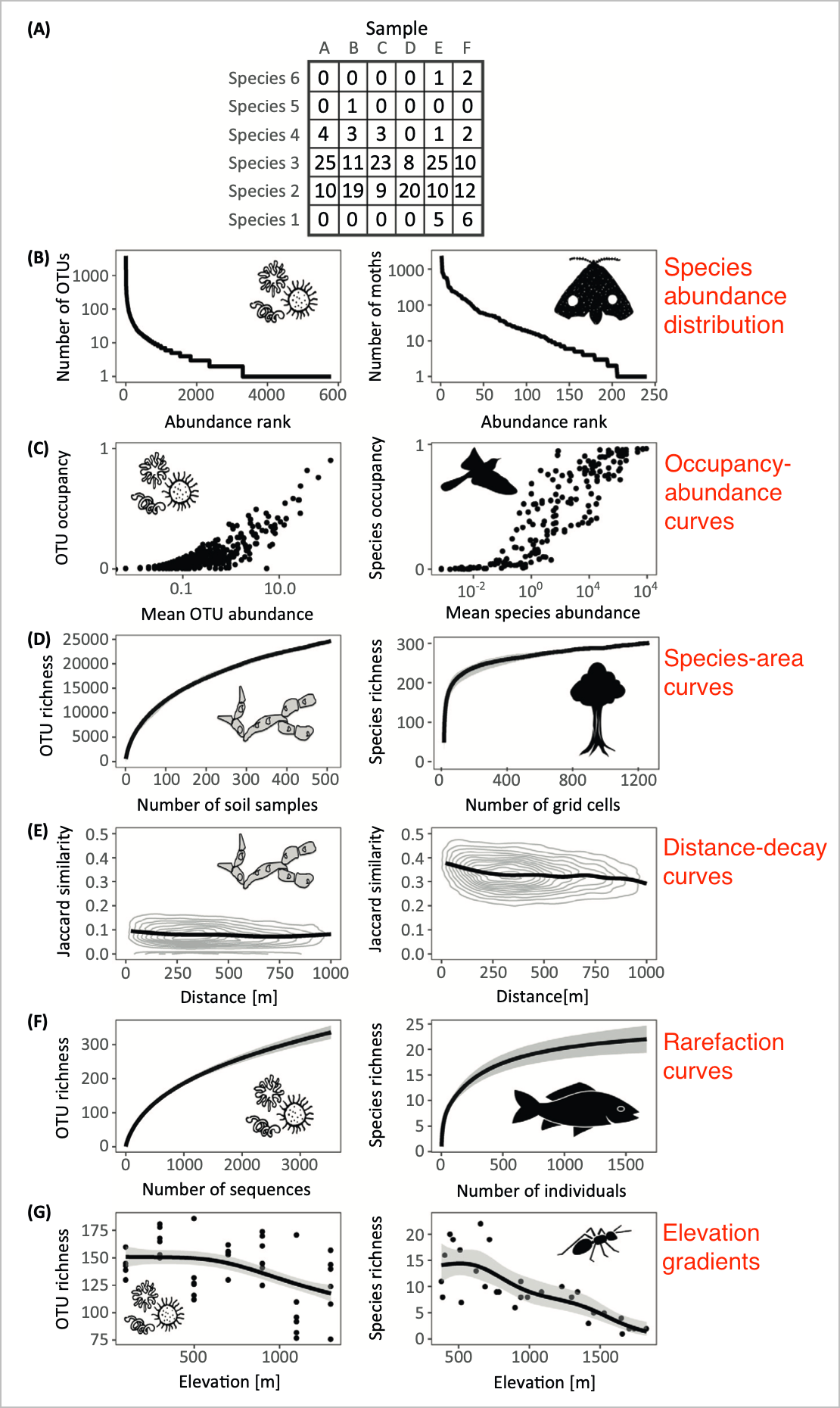
You will already be familiar with the paper by Shade et al. (2018). Several kinds of ecological patterns are mentioned in the paper, and they can be derived from a species table with abundance data (but not presence-absence data!). The patterns that can be derived from such a table include (see Figure 1 below), and they are as follows:

• Species-abundance distribution
• Occupancy-abundance curves
• Species-area curves
• Rarefaction curves
• Distance-decay curves
• Elevation gradients

Figure 1: Species distribution curves by Shade et al. (2018). Note that this figure starts with a species table where the species are arranged down the rows and the sites along the variables (columns). I, and also the vegan package, require that the species are down the columns (called variables) and the sites (or samples) are along the rows. This is the convention that will be used throughout this module.

Species Abundance Distribution

Species Abundance Distribution (SAD) describes how individuals are distributed among all the species within our sampled community. It tells us about the patterns of species dominance and rarity—this information relates to a more nuanced understanding of ecological dynamics, community structure, and the mechanisms driving biodiversity. SAD curves can be made for any community for which we have species lists with their abundances.

The first form of SAD is the one given by Shade et al. (2018), which shows the number of individuals (N) of each species in a sample. It is formed by log(N) (on y) as a function of species rank (on x), with species ranked 1 most abundant and plotted on the left and decreasing to less abundant species on the right. Matthews and Whittaker (2015) call this form of SAD a Rank Abundance Distribution (RAD) curve. The profile of this relationship can be variable, but in general it shows that only a few species attain a high abundance while the majority of them are rare. This is a typical pattern in most communities and is often referred to as a log-normal distribution, but some other models can also be used to describe these SADs. The type of model applied to a SAD curve may reveal different ecological processes and mechanisms. Matthews and Whittaker (2015) argue that the form of the SAD and the model that describes its form can be used to develop suitable ecosystem health assessment insights and develop applicable conservation and management strategies.

References

Matthews TJ, Whittaker RJ (2015) On the species abundance distribution in applied ecology and biodiversity management. Journal of Applied Ecology 52:443–454.

Shade A, Dunn RR, Blowes SA, Keil P, Bohannan BJ, Herrmann M, Küsel K, Lennon JT, Sanders NJ, Storch D, others (2018) Macroecology to unite all life, large and small. Trends in ecology & evolution 33:731–744.