Lecture 2a. Ecological Gradients

This material must be reviewed by BCB743 students in Week 1 of Quantitative Ecology.
Robert H. Whittaker’s Role in Understanding Community Formation
Robert H. Whittaker (1920-1980) was instrumental in shaping our understanding of ecological gradients and their role in species community formation. He challenged the prevailing Clementsian view of his time of communities as discrete, interdependent units, and instead proposed the “individualistic hypothesis” (Whittaker 1953). This hypothesis posited that species respond individually to environmental gradients, resulting in gradual shifts in community composition along these gradients.
Whittaker undertook extensive field research in diverse ecosystems, from the Great Smoky Mountains to the Siskiyou Mountains. This work provided strong empirical support for his hypothesis (Whittaker 1967). He developed the “gradient analysis” method, a quantitative approach to studying species distributions along environmental gradients, which became a cornerstone of modern community ecology.
Whittaker’s placed community ecology onto a new trajectory and shifted the focus from discrete community types to the continuous variation of species along environmental gradients. This shift is continuing to have deep implications for our understanding of biodiversity patterns, ecosystem functioning, and conservation strategies.
Environmental Gradients
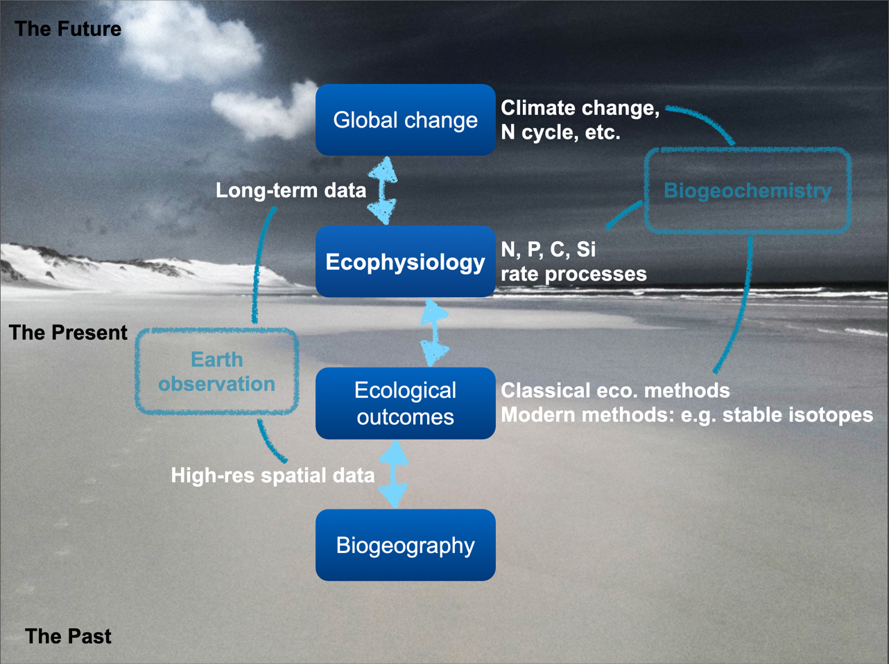
Environmental gradients exist across space and time and link biodiversity outcomes, which we may measure as structure and function, to environmental properties {Figure 1). These gradients can be observed through Earth observation technologies, such as satellite remote sensing, which provide high-resolution spatial data essential for understanding biogeography. Biogeographical patterns help us discern how species distributions and community compositions vary in response to different environmental factors such as temperature, precipitation, and nutrient availability. We refer to these environmental factors as drivers when they affect ecological—and ultimately, biogeographical—outcomes.
As we move from present to future scenarios, the data collected enable us to use ecophysiological principles: that is, we use our understanding of physiological processes of organisms and how they adapt to changing environments. Long-term data are crucial for understanding global change processes, such as climate change and nutrient cycles such as those involving N, P, C, and Si, for example. These processes impact ecological outcomes by altering ecosystem structure and function, and can be studied using both classical ecological methods and modern techniques like stable isotopes. These outcomes feed back into biogeochemistry, linking the cycles of key elements to broader ecological and environmental changes. This interconnected approach can help us predict how ecosystems might respond to future environmental shifts, emphasising the importance of integrating data across temporal and spatial scales.
The Unimodal Model
The ‘unimodal’ model (sensu Whittaker 1967) is a core concept in ecology. It provides a framework for understanding how species and communities are distributed along environmental gradients and offers an intuitive explanation for the patterns we observe in nature.
The unimodal model posits that the relationship between a species’ abundance (or other measures such as biomass or relative frequency) and its position along an environmental gradient follows a unimodal function. This means that the abundance of a species typically peaks at a specific point along the gradient where the conditions are ‘just right’ (to quote Goldilocks) and decreases as conditions deviate from this optimum in either direction.
The model implies that each species has a unique set of optimal conditions under which it thrives and attains maximal abundance. This ‘sweet spot’ represents the ideal combination of environmental factors for that particular species. As conditions move away from this optimum, whether becoming too hot or too cold, too wet or too dry, the species’ abundance decreases. This creates a characteristic bell-shaped curve (Figure 2) when plotting abundance against the environmental gradient.
Show the code
library(coenocliner)
set.seed(666)
M <- 3                                     # number of species
ming <- 3.5                                # gradient minimum...
maxg <- 7                                  # ...and maximum
locs <- seq(ming, maxg, length = 100)      # gradient locations
opt  <- runif(M, min = ming, max = maxg)   # species optima
tol  <- rep(0.25, M)                       # species tolerances
h    <- ceiling(rlnorm(M, meanlog = 3))    # max abundances
pars <- cbind(opt = opt, tol = tol, h = h) # put in a matrix

mu <- coenocline(locs, responseModel = "gaussian", params = pars,
                 expectation = TRUE)

matplot(locs, mu, lty = "solid", type = "l", xlab = "pH", ylab = "Abundance")
The unimodal model is simple to understand and has a broad applicability. It’s trivial to conceptualise how species come to be arranged or sorted along gradients based on their individual optimal conditions and tolerance ranges. This sorting effect explains why we often observe distinct changes in species composition as we move along environmental gradients, such as elevation in mountains or moisture in transitions from wetlands to uplands, or even across wider regional gradients such as along a coastline influenced by a western boundary current (e.g. Agulhas Current) or east to west across South Africa. This gives rise to the ideas of distance-decay relationships, community structuring along elevation gradients, and species turnover, for all of which the outcome can be measured as beta diversity.
In real-world ecosystems, however, multiple gradients co-exist simultaneously and the situation may be more complex than alluded to in Figure 2. Species are responding not just to one environmental factor, but to a complex interplay of various gradients. These might include temperature, precipitation, soil pH, nutrient availability, and many others. As a result, communities—collections of species coexisting in a given area—are formed within this multidimensional ‘space’ of gradients. Please see the section on coenoplanes and coenospaces for more information. To complicate things further, many types of biotic interactions (e.g. competition, predation, mutualism) can also influence species distributions and community assembly.
Fundamental and Realised Niches
The formation of communities in this gradient space can be conceptualised as the outcome of multiple interacting unimodal species-environment relationships, modulated by complex biological interactions. Each species in the community occupies a position that reflects its response to various environmental gradients, shaped by its physiological tolerances, competitive abilities, and other biotic factors. This interplay leads to the complex patterns of species composition and diversity we observe in nature.
To fully understand this process, we must consider the concepts of fundamental and realised niches. The fundamental niche represents the full range of environmental conditions under which a species could potentially thrive in the absence of biotic interactions. In the context of the unimodal model, this would correspond to the species’ theoretical response curves along various environmental gradients.
However, in real ecosystems, species rarely occupy their entire fundamental niche. Instead, they occupy a realised niche, which is typically a subset of the fundamental niche. The realised niche is shaped by biotic interactions such as competition, predation, and mutualism, as well as by dispersal limitations and historical factors. In the gradient space, a species’ realised niche is represented by its actual measurable distribution and abundance patterns.
The interaction between fundamental and realised niches adds layers of complexity to community formation. Competition may lead to niche compression, where species occupy narrower niches than they are physiologically capable of. Conversely, in the absence of competitors or predators, species might experience niche expansion. Over time, niche differentiation can occur as species evolve to reduce competition, potentially altering their response to environmental gradients.
Moreover, some species exhibit niche plasticity, adjusting their ecological roles in response to environmental changes or biotic pressures. Others engage in niche construction, actively modifying their environment and thereby altering the gradient space for themselves and other species.
Understanding these dynamics is important if we wish to interpret the complex patterns we observe and measure in nature. ‘Community assembly’ (note, not implying a deliberate act) is not simply a passive response to existing gradients, but a dynamic process involving adaptation, competition, and environmental modification. We must consider both abiotic factors, as emphasised in the unimodal model, and the various kinds of biotic interactions, as highlighted by the concept of realised niches.
The Unified Neutral Theory of Biodiversity
An alternative (or complementary?) hypothesis for community formation—which we will not cover too much but you are nevertheless required to understand the basic premise of—is the Unified Neutral Theory of Biodiversity (UNTB). This theory posits that species in a community are functionally equivalent and that their relative abundances are determined by stochastic processes rather than by their individual traits or interactions. In other words, the UNTB suggests that all species are ecologically equivalent and that community composition is the result of random dispersal, speciation, and extinction events.
Please consult the following references for more information on the UNTB:
- Hubbell (2005)
- Hubbell (2011)
- Rosindell et al. (2012)
- Neutral Theory of Species Diversity
References
Reuse
Citation
@online{smit,_a._j.2024,
  author = {Smit, A. J.,},
  title = {Lecture 2a. {Ecological} {Gradients}},
  date = {2024-07-22},
  url = {http://tangledbank.netlify.app/BDC334/L02a-gradients.html},
  langid = {en}
}